Curve fitting Using Python

AIM

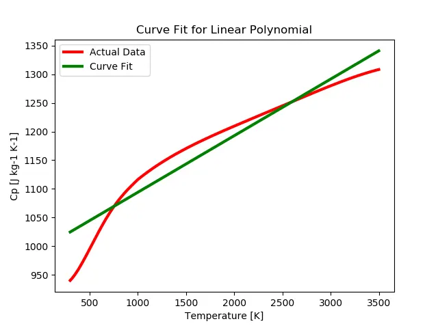
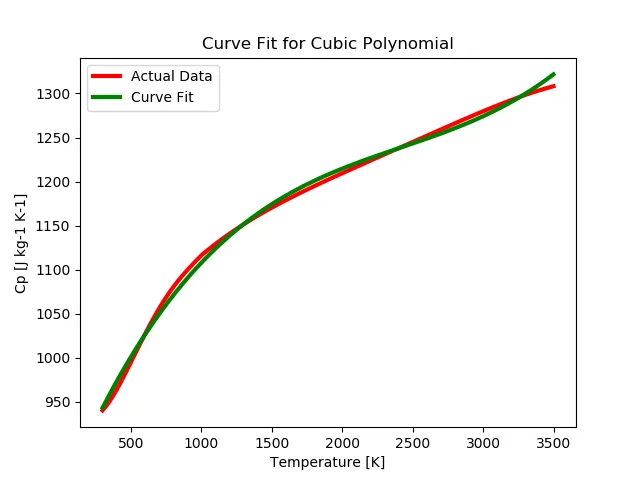
To write code to fit a linear and cubic polynomial for the Cp data and explain the following Questions

1. What do popt and pcov mean?

2. What does np.array(temperature) do?

3. What does the * in *popt mean?

4. What needs to be done in order to make the curve fit perfectly?

Theory:-

What is Curve Fitting?

Curve fitting is the process of constructing a curve, or mathematical functions, which possess the closest proximity to the real series of data. By curve fitting, we can mathematically construct the functional relationship between the observed dataset and parameter values, etc. It is highly effective in the mathematical modeling of some natural processes.

1. Popt and Pcov:-

• Popt is an array returned by the curve fit function that contains the optimized value of the parameters of the function passed to curve_fit. In this case, it is an array containing the optimum values of the coefficients of the function in order to obtain the plot that best fits the given data.
• Pcov is a matrix whose diagonal components contain the change of popt which can be removed and its square root gives the standard deviation to blunder from the Actual Data points.

2. np.array(temperature):-

• It allows to perform any mathematical operations (like addition or subtraction) either on every element of an array or between the arrays, we need to import the numpy library.
• Here we called the numpy module but to use it we are using (np) because we imported the numpy module is as "import numpy as np". The temperature is an array because it contains more than one value, so we need to define it first. hence using an array(temperature) here.

3. * in *popt

* refer to the values generated and stored in the popt array and helps us to call values for (a,b,c)

Program:-

Python Program to fit a linear and cubic polynomial for the Cp data

"""
 Curve fit program
 By Saurabh Nambiar

"""
import math
import matplotlib.pyplot as plt
import numpy as np
from scipy.optimize import curve_fit as cfit

def linear_poly(t,a,b):
	return a*t + b

def cubic_poly(t,a,b,c,d):
	return a*pow(t,3) + b*pow(t,2) + c*t + d

def read_file():
	temperature = []
	cp = []
	for line in open('data','r'):
		values = line.split(',')
		temperature.append(float(values[0]))
		cp.append(float(values[1]))
	return [temperature,cp]

temperature,cp = read_file()
#Considering the Linear Polynomial
popt1,pcov1 = cfit(linear_poly,temperature,cp)
fit_cp1 = linear_poly(np.array(temperature),*popt1)

#Considering cubic Polynomial
popt2,pcov2 = cfit(cubic_poly,temperature,cp)
fit_cp2 = cubic_poly(np.array(temperature),*popt2)

#plotting
#linear fit
plt.figure(1)
plt.plot(temperature,cp,color='red',linewidth=3)
plt.plot(temperature,fit_cp1,color='green',linewidth=3)
plt.legend(['Actual Data','Curve Fit'])
plt.xlabel('Temperature [K]')
plt.ylabel('Cp [J kg-1 K-1]')
plt.title('Curve Fit for Linear Polynomial')
plt.savefig('linear.png')
#cubic curve fit
plt.figure(2)
plt.plot(temperature,cp,color='red',linewidth=3)
plt.plot(temperature,fit_cp2,color='green',linewidth=3)
plt.legend(['Actual Data','Curve Fit'])
plt.xlabel('Temperature [K]')
plt.ylabel('Cp [J kg-1 K-1]')
plt.title('Curve Fit for Cubic Polynomial')
plt.savefig('cubic.png')

plt.show()

Results:-

4. Best curve fit

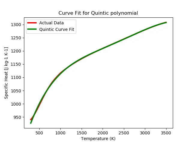
A curve is said to be the best fit when it passes through a scatter plot of data while best expressing the relationships between the points. This can be achived by using Heigher order Polynomials in this case we use a quintic polynomial.

"""
Code for best fit
By Saurabh Nambiar

"""
import math
import matplotlib.pyplot as plt
import numpy as np 
from scipy.optimize import curve_fit as cfit

# Curve fit function for Quintic polynomial
def quintic_poly(t,a,b,c,d,e,f):
	return a*pow(t,5) + b*pow(t,4) + c*pow(t,3) + d*pow(t,2) + e*t + f

# Reading Thermodynamic Data file
def read_file():
	temperature = []
	cp = []

	for line in open('data','r'):
		values = line.split(',')
		temperature.append(float(values[0]))
		cp.append(float(values[1]))

	return[temperature,cp]

# Main Program 
temperature,cp = read_file()
popt,pcov = cfit(quintic_poly,temperature,cp)
fit_cp5 = quintic_poly(np.array(temperature), *popt)

plt.plot(temperature,cp,color='red',linewidth=3)
plt.plot(temperature,fit_cp5,color='green',linewidth=3)
plt.title('Curve Fit for Quintic polynomial')
plt.legend(['Actual Data','Quintic Curve Fit'])
plt.xlabel('Temperature [K]')
plt.ylabel('Specific Heat [J kg-1 K-1]')
plt.savefig('quintic.png')
plt.show()

Results

Conclusion-

• When we use Linear Polynomial we get a bad fit but we can observe that both (actual Data and linear CF) are on the same direction.
• We we curve fir for cubic polynomial we can observe that we get comparitively better results this can be termed as a good fit but not a perfect fit.
• We get almost a perfect fit when we use hiegher order polynomials, this can be obtained up to a certain limit, to make the fit more perfect we can split the temprature range and use the temprature obtained with diffrent orders polynomial this method is called Split Wise method, This method is very accurate.

References:-

https://skill-lync.com/projects/Curve-Fitting-and-criterion-to-choose-best-fit-41860

l