Curve Fitting using Python

CURVE FITTING AND FITNESS CHARACTERISTICS

Objective:

1. To fit a linear & cubic polynomial curve for Cp (specific heat) with the range of temperature.
2. Explain the parameters to measure the fitness characteristic of a curve.
3. Also discuss how to make a curve perfect fit, best fit, and what could be done to improve the cube fit.

Theory:

Introduction to curve fitting:

Curve fitting is a method of construction of a curve or a function by capturing a trend in the data which possesses the highest correlation to the real data. By doing so we can develop a mathematical relation between the observed values and parameter values.

This method has very high use in engineering application and science, so the question arises 'why it is required to study?'

• To carry out system simulation & optimization.
• To determine the value of properties of intermediate points.
• To do trend analysis.
• For hypothesis testing.

suppose we have a set of `n` data such as:

`(y1,x1),(y2,x2),(y3,x3)...........(yn,xn)`

The first step is to plot this data and postulate a function form `f(x)` to describe the general trend from those data.

some simple function commonly used are:

• straight line: `f(x) = ax + b`
• parabola: `f(x) = ax2 + bx + c`
• polynomial: `f(x) = a underset (m)x^m + aunderset(m−1)x^ (m−1) + · · · + a underset 2x ^2 + a1x + a0`
• Exponential: `f(x) = c exp^(ax)`
• Gaussian, e.g. `f(x) = c exp^(−bx2)`
• sine or cosine, e.g. `f(x) = a cos(bx) + c`

A curve fit can be of two type either:

1. Perfect/Exact Fit
2. Best fit

Perfect fit:

• curve passes through every data points.
• suitable for small No. of parameters e.g. `h=f(t,p)` (includes property data &calibration data).

Best fit:

• The curve does not passes through every point.
• suitable for large no. of parameters. e.g. Regression in engineering problem, Nusselt no. correlation `(Nu=aRe^bPr^c)`.
• for an overdeterminent system where No. of data points are too many & not highly accurate(error).

Basic fundamental

we get values at discrete points & convert all this into an equation form , so that it can be used for an entire range of systems.

Method of Perfect/ Exact fit(Interpolation)

1. Polynomial interpolation
2. Lagrange interpolation(Imp.)
3. Newton's divide difference polynomial
4. Spline fit

Method of best fit

1. Polynoimial- `[y=a+bx+cx^2]`
2. Eponential- `[y=ae^(bt)]`
3. power law- `[y =a x^b]`

................e.t.c

Goodness of a Fit

Regression:

It is a method of describing the relationship between one dependent variable (y) with series of changing variables which are known as an independent variable, such that it is best fit that satisfies entire range of the independent variables.

In order to choose the best fit we follow the Least Square Method.

it is the procedure of finding the best fitting curve in set of data points by minimizing the sum of the Square of the Offset(Residual) of the point on the curve.

The sum of the squares of the offsets is used instead of the offset absolute values, to permit the residuals to be treated as a continuously differentiable quantity.

If we use higher exponents it would be harder to find the minimum value(s), and we could find possibly nonunique minimums. we used squared error because it gives us a minimum that is easy to find and is guaranteed to be the only minimum.

Type of sum of squares

1. sum of squares of Error(residual) (SSE)or(RSS)
2. sum of squares of Regressions (SSR) or(ESS)
3. Total sum of squares (TSS)
4. Root mean square error (RMSE)

1) Sum of square of error(SSE): it is the sum of the squares of the residue i.e. the sqaure of the difference of the data and the fit, which is represented by :

`SSE=sum_(i=1)^n[(y_i-f(x_i))^2]`

2) Sum of square of Regressions(SSR): It is the sum of the squares of the regression i.e. the sqaure of the difference of the value of dependent variable`(f(x_i))` and mean of the sample data`(mu)` ,which is represented by :

`SSR=sum_(i=1)^n[(f(x_i)- mu)^2]`

3) Total Sum of square(TSS): It is the sum of the squares of the differences between the sample data`(y_i)` to the mean of the sample data `(mu)`,which is represented by :

`TSS=sum_(i=1)^n[(y_i- mu)^2]`= SSE+SSR`

R-squared value: It is the called the cofficient of determinent`(R^2)`. It tells about the goodness of the fit. It tells how fell the fit is in correlation to the set of data.

`R^2= (SSR)/(SST)`

Note:

• Higher the value of R higher better is the fit.
• Value of R ranges from [o-1] .
• More R value approaches 1( `R->1`) better fit.

If R-squared value is greater than 0.95 the fit is assumed to be good

4) Root Mean Square Error: It is the fit standard error or standard error of the regression. it is the root of the average of the standard error or standard deviation. lower the value better is the fit.

`RMSE=root( )((sum_(i=1)^n[(y_i-f(x_i))^2])/n) =root()((SSE)/n)`

What does popt and pcov mean?

pout: 1D array- optimal value for the parameter so that the sum of the squared residual of f(xdata,*pout)- ydata is minimized

In simple if contains the coefficients of the n order of equation

eg. y=ax+b where a and b are the coefficients

pcov: 2D array- The estimated covariance of the popt. The diagonals provide the variance of the parameter estimate. To compute one standard deviation error on the parameters use perr = np.sqrt(np.diag(pcov)).

* symbol before a variable means eg. *popt

A single asterisk as used in function declaration allows a variable number of arguments passed from the calling environment. Inside the function, it behaves as a tuple.

*- unpacks a list or tuple into position arguments

**- unpacks a dictionary into keyword arguments

What does np.array(temperature) do?

While reading line by line from the 'DATA' file the temperature column is saved as a list so np.array(temperature) will convert the list to array type. The np.array is preferred over the list as it is much much faster and convenient for applying np functions.

Python code to fit a cubic & linear fit curve

import numpy as np 
import matplotlib.pyplot as plt 
from scipy.optimize import curve_fit

# curve fit function
def func(t,a,b,c,d):
	return a*pow(t,3) +b*t*t + c*t+d
def func1(t,a,b):
	return a*t +b

#Reading the data file properties.
def read_file():
	temperature=[]
	cp= []
	for line in open('data','r'):
		value=line.split(',')	
		temperature.append(float(value[0]))
		cp.append(float(value[1]))

	return[temperature,cp]

# Main Program
temperature,cp = read_file()
popt,pcov = curve_fit(func, temperature, cp)
popt1,pcov1 = curve_fit(func1, temperature, cp)
#predicted Cp value for Cubic equationfrom function func
fit_cp= func(np.array(temperature), *popt)
#predicted Cp value for Linear equation from function func1
fit_cp1= func1(np.array(temperature), *popt1)

#plotting Cubic fit curve 
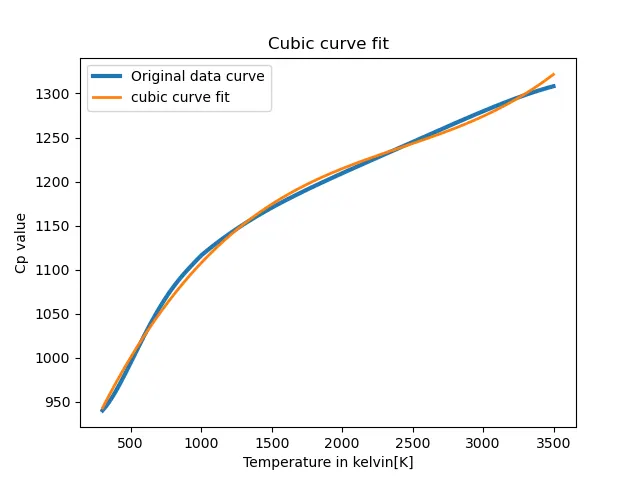
plt.plot(temperature,cp,linewidth=3)
plt.plot(temperature, fit_cp,linewidth=2)
plt.xlabel('Temperature in kelvin[K]')
plt.ylabel('Cp value')
plt.savefig( "plotcubic")
plt.legend(['Original data curve','cubic curve fit'])
plt.title('cubic curve fit')
plt.show()
plt.close()

#plotting linear fit curve  
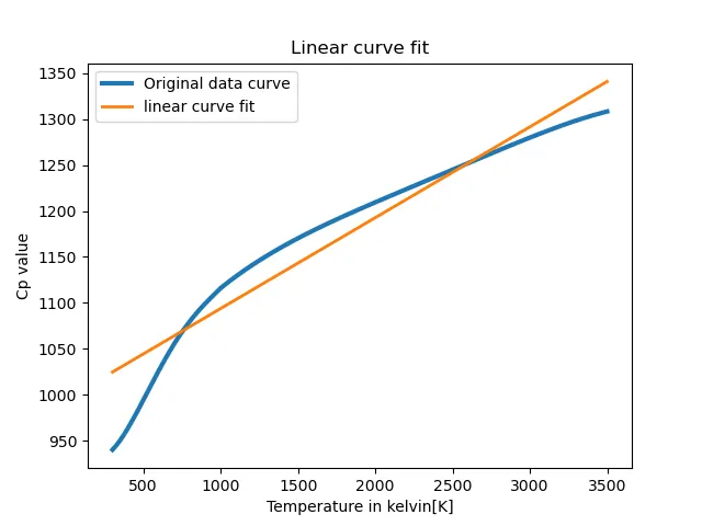
plt.plot(temperature,cp,linewidth=3)
plt.plot(temperature, fit_cp1,linewidth=2)
plt.xlabel('Temperature in kelvin[K]')
plt.ylabel('Cp value')
plt.legend(['Original data curve','linear curve fit'])
plt.title('linear curve fit')
plt.savefig( "plotlinear")
plt.show()
plt.close()

Result:

1) Cubic Fit Curve

2) Linear Fit Curve

What needs to be done in order to make the curve fit perfect?

In order to make the curve perfectly fit, we can split the original curve into small 10 sections (as shown below) and try to get the coefficient value for all the 10 curves(quadratic) such that it perfectly fits the original curve.

Show empirically as to how well your curve has been fit.

As I explained in the introduction part the R-square value, so the value of the R-square tells about the goodness of fit where if the value approaches 1(in real condition>0.92) is preferred to be a better fit.

`R^2= (SSR)/(SST)`

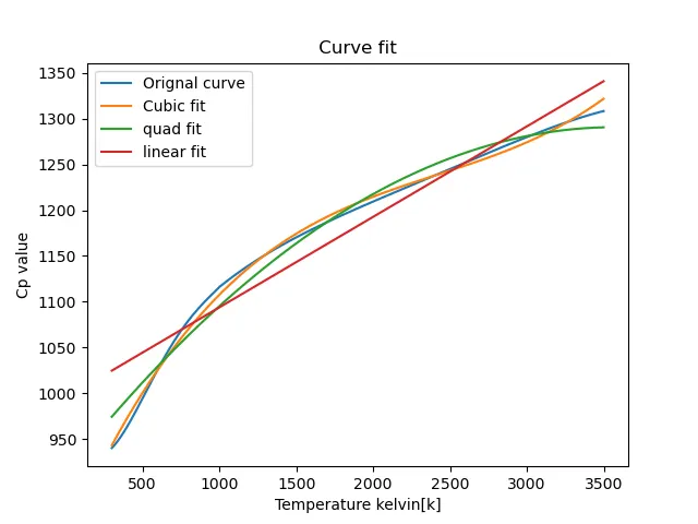
There is a different method that I have used for the curve fit in python using 'partial function' and 'pandas csv reader' to read a file

import numpy as np 
import pandas as pd
import matplotlib.pyplot as plt 
from scipy.optimize import curve_fit
from functools import partial
import pdb

# CURVE FIT FUNCTION

# partial function defination
def cubic(coef, t):
	return coef[0]*t*t*t + coef[1]*t*t + coef[2]*t + coef[3]
def quad(coef, t):
	return coef[0]*t*t + coef[1]*t + coef[2]
def linear(coef, t):
	return coef[0]*t+ coef[1]

# function defining curve order.
def func1(t, a, b, c, d):
	return a*t*t*t + b*t*t + c*t + d
def func2(t, a, b, c):
	return a*t*t + b*t + c
def func3 (t, a, b):
	return a*t + b

# Main Program

# Read csv file using pandas csv reader in a single go.
data = pd.read_csv('data', header=None) # no need of a for loop 
print(data)

# cofficient calculation of cubic, quad, linear orders 
popt1, pcov1 = curve_fit(func1, data[0], data[1])
popt2, pcov2 = curve_fit(func2, data[0], data[1])
popt3, pcov3 = curve_fit(func3, data[0], data[1])

# partial function calling  
cp_func1 = partial(cubic, popt1)
cp_func2 = partial(quad, popt2)
cp_func3 = partial(linear, popt3)

# perdicted cp value for cubic, quadratic and linear fit
cp_projected1 = data[0].apply(cp_func1)
cp_projected2 = data[0].apply(cp_func2)
cp_projected3 = data[0].apply(cp_func3)

# plotting the all curve in a single graph  
plt.plot(data[0],data[1])
plt.plot(data[0],cp_projected1)
plt.plot(data[0],cp_projected2)
plt.plot(data[0],cp_projected3)
plt.title(' Curve fit ')
plt.legend(['Orignal curve','Cubic fit','quad fit', 'linear fit'])
plt.xlabel('Temperature kelvin[k]')
plt.ylabel('Cp value')
plt.savefig( "plotall")

plt.show()

Result