Curve fitting

Aim

• Create a program for Linear and Cubic polynomial curve fit.
• Plat the actual data and predicted data on the plot to compare both.
• Find out error between actual data and predicted one.
• Answer the following questions
• [1] What does popt and pcov mean?
• [2] What does np.array(temperature) do?
• [3] What does the * in *popt mean?
• [4] Write code to fit a linear and cubic polynomial fo the Cp data. Explain if your results are good or bad.
• [5] What needs to be done in order to make the curve fit perfect?

Objective:

• Study about curve fit and its use in codding.
• Write the code for linear and cubic polynomial curve fit.
• Plot the predicted data of curve fit and actual data on same figure to compare the results.
• Write down the codes for error and variation in curve fit.
• Explain all the codes and write down the answer of each questions.

Curve fitting:-

In given set of observed data, we try to fit best curve through those data points, called the curve fitting.

This can be done it by using various equation which advantage is that we can find the values at the points, we haven’t observed by just substituting that value in the equation. It can be easily misunderstood by Interpolation method but this is not exactly the interpolation. As in interpolation, we are restricted to finding unobserved values only between two observed points, using a pre-defined curve fit between those two points. In curve fitting we want some approximate values, in between observed data points.

Curve Fit Analysis:-

We will use our typical step-by-step approach. We’ll start with the Linear fit, and not long after, we will be dealing with the Polynomial curve fit. And then, we will learn how to build a Curve fit, how to interpret it and how to compare different models.

The Process of Creating Linear curve fit goes like this.

1. Firstly, we get sample data;
2. Then, we can design a model that explains the data;
3. Finally, we use the model that we have developed to make a prediction for the whole cp data Using linear and cubic polynomial method.

A Curve fit Example

Think about the following equation:In steam table, Heat capacity (cp) is depend upon changes in temperature(T). The dependant variable is Heat capacity(cp), while the independent variable is temperature(T).

In order to start programming, first, we are going to import required library for this particulate problem.

import numpy as np 
import matplotlib.pyplot as plt
from scipy.optimize import curve_fit

Now we create function for each polynomial equation.

[1] For linear polynomial or first degree polynomial the equation is:-

`ax + b`

Then the function will be:-

# First degree polynomial (Linear polynomials)
def Linear(t,a,b):
	return a*t + b

[2] For quadratic polynomials or second order polynomial the equation will be:-

`ax^2 + bx + c`

Then the function for second order polynomial will be:-

# Second degree polynomial (Quadratic polynomials)
def Quadratic(t,a,b,c):
	return a*(t**2) + b*t + c

[3] for Cubic polynomial or third degree polynomial the equation will be:-

`ax^3 + bx^2 + cx +d`

Then the function for cubic polynomial will be:-

# Third degree polynomial (Cubic polynomials)
def Cubic(t,a,b,c,d):
	return a*(t**3) + b*(t**2) + c*t + d

After setting function we will call the cp and temperature data from data file by defining function and applying for we are going to store each data line by line in their respective array.

To store their value separately split line by “,” in two part assign first value “value 0” as temperature and next value “value 1” as cp.

Use return to read all the line step by step and store values in empty array accordingly.

Following are the codes to extract data from file and store in empty array.

# Reading thermodynamic data file
def read_file():
	temperature=[]
	cp = []
	for line in open('data','r'):
		values = line.split(',')
		temperature.append(float(values[0]))
		cp.append(float(values[1]))
	return [temperature, cp]

Next, we are going to plot 4 graph for curve fitting to compare best fit. In order to do that we are going to plot 4 subplot in one figure window.

So create figure and mention its size. In this case, it is 12`xx`11 and then arrange 4 plot namely ax1, ax2, ax3, and ax4 by providing proper grid location in figure window.

Lastly give main heading using fig.suptitle as ‘curve fit’

# Subplot for the figure1 and figure two
fig = plt.figure(figsize=(12,11),linewidth=6, edgecolor="k")
ax1 = plt.subplot2grid((12, 11), (0, 0), colspan=5,rowspan=5)
ax2 = plt.subplot2grid((12, 11), (0, 6), colspan=5,rowspan=5)
ax3 = plt.subplot2grid((12, 11), (7, 0), colspan=5,rowspan=5)
ax4 = plt.subplot2grid((12, 11), (7, 6), colspan=5,rowspan=5)
fig.suptitle('Curve fitting',size='22',weight='bold',color='m')

Output for the above codes:-

From here, we can start our main coding by curve fitting and first we are going to call the read_file() function to call cp and temperatures values which is out actual value using this value we are going to find out our cure fit.

temperature, cp = read_file()

Here we are using scipy library for optimization for best cure fit.

Which is use as “popt, pcov = curve_fit(func, xdata, ydata)”

Where,

func - the callable function that we created using different type of polynomial equation.

xdata- the The independent variable where the data is measured. Should usually be an M-length sequence or an (k,M)-shaped array for functions with k predictors, but can actually be any object.

Ydata - The dependent data, a length M array - nominally f(xdata,…)

popt (1-D array) - Optimal values for the parameters so that the sum of the squared residuals of f(xdata, *popt)-ydata in minimize.

Pcov(2-D array) - The estimated covariance of popt. The diagonals provide the variance of the parameter estimate.

Predicted_array by using function is calculated by using xdata and optimum value for the co-efficient of the equation. In this case, ‘*’ in ‘*popt’ is used to pass all the required positional arguments to determine function means pass all the coefficients value from function.

Predicted_y_array = func(np.array(xdata), *popt)

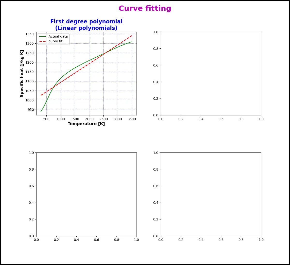
After that, we can plot all the value of cp and predicted cp in the first plot.

popt, pcov = curve_fit(Linear, temperature, cp)
fit_cp_Linear = Linear(np.array(temperature), *popt)

ax1.plot(temperature, cp, color='g', linewidth='1.5')
ax1.plot(temperature, fit_cp_Linear,'--', color='r',linewidth='2')
ax1.legend(['Actual data','curve fit'])
ax1.set_title('First degree polynomial\n(Linear polynomials)',color='b',size='16',weight='bold')
ax1.set_xlabel('Temperature [K]',size='12',weight='bold')
ax1.set_ylabel('Specific heat [J/kg K]',size='12',weight='bold')
ax1.grid(color='b',linestyle=':',linewidth='0.5')

Output for the above codes:-

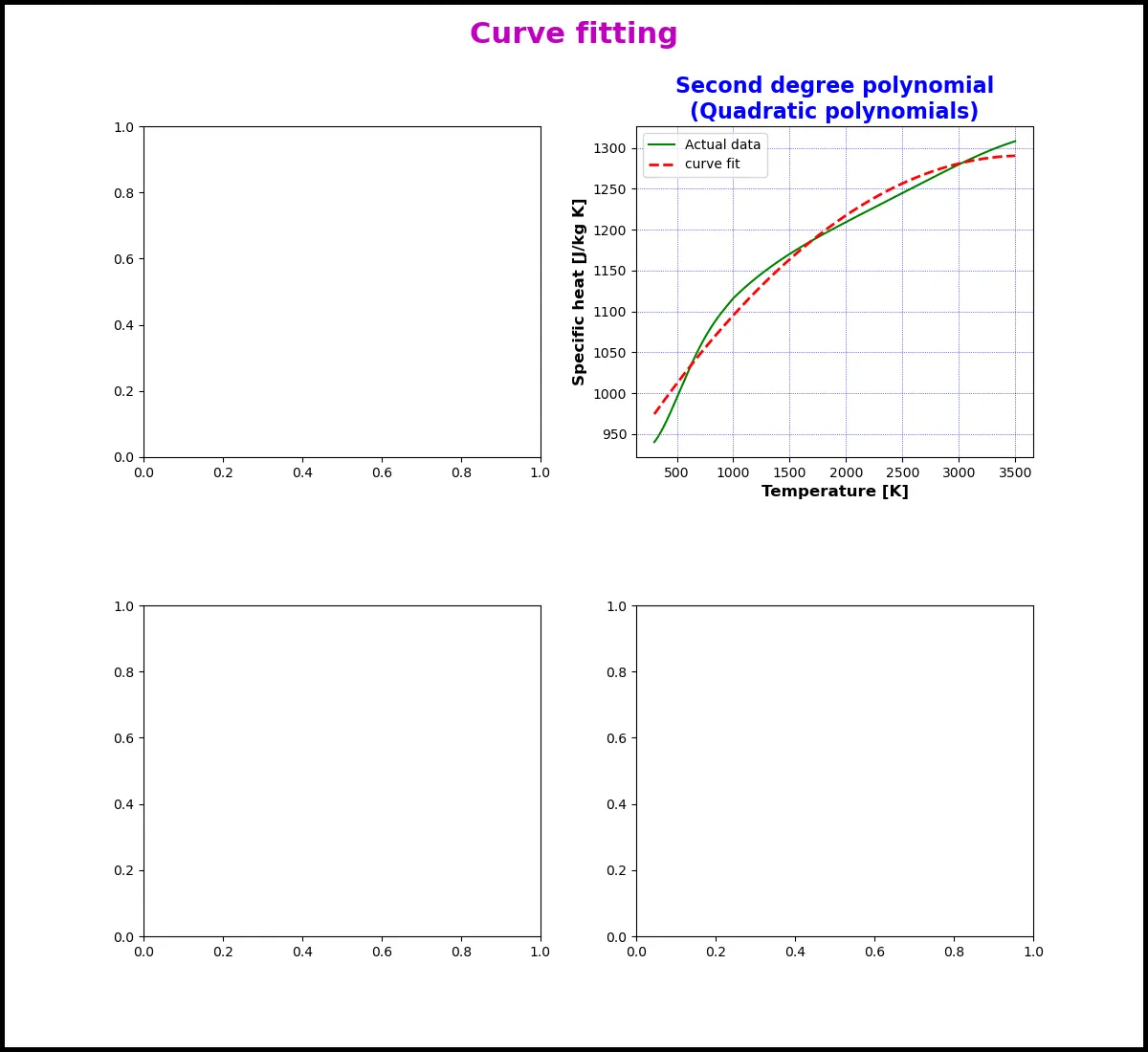
By using same technique, we will use following codes to calculate quadratic polynomial curve fit.

popt, pcov = curve_fit(Quadratic, temperature, cp)
fit_cp_Quadratic = Quadratic(np.array(temperature), *popt)

ax2.plot(temperature, cp, color='g', linewidth='1.5')
ax2.plot(temperature, fit_cp_Quadratic,'--', color='r',linewidth='2')
ax2.legend(['Actual data','curve fit'])
ax2.set_title('Second degree polynomial\n(Quadratic polynomials)',color='b',size='16',weight='bold')
ax2.set_xlabel('Temperature [K]',size='12',weight='bold')
ax2.set_ylabel('Specific heat [J/kg K]',size='12',weight='bold')
ax2.grid(color='b',linestyle=':',linewidth='0.5')

Output for the above program

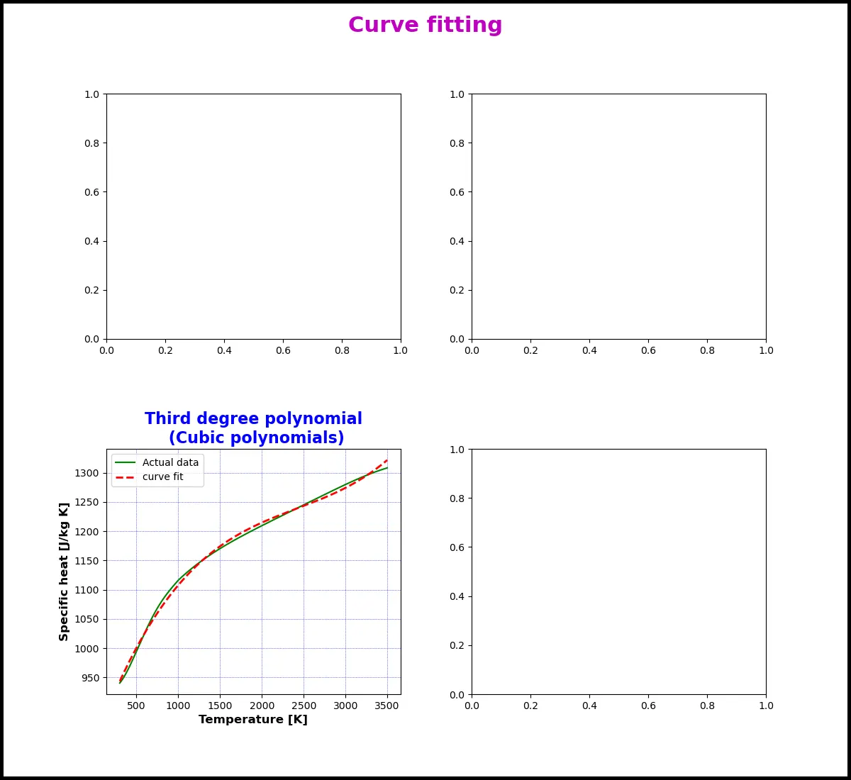
Also similar way we are going to plot a graph for the cubic polynomial function using following codes.

popt, pcov = curve_fit(Cubic, temperature, cp)
fit_cp_Cubic = Cubic(np.array(temperature), *popt)

ax3.plot(temperature, cp, color='g', linewidth='1.5')
ax3.plot(temperature, fit_cp_Cubic,'--', color='r',linewidth='2')
ax3.legend(['Actual data','curve fit'])
ax3.set_title('Third degree polynomial\n (Cubic polynomials)',color='b',size='16',weight='bold')
ax3.set_xlabel('Temperature [K]',size='12',weight='bold')
ax3.set_ylabel('Specific heat [J/kg K]',size='12',weight='bold')
ax3.grid(color='b',linestyle=':',linewidth='0.5')

Output for the above codes.

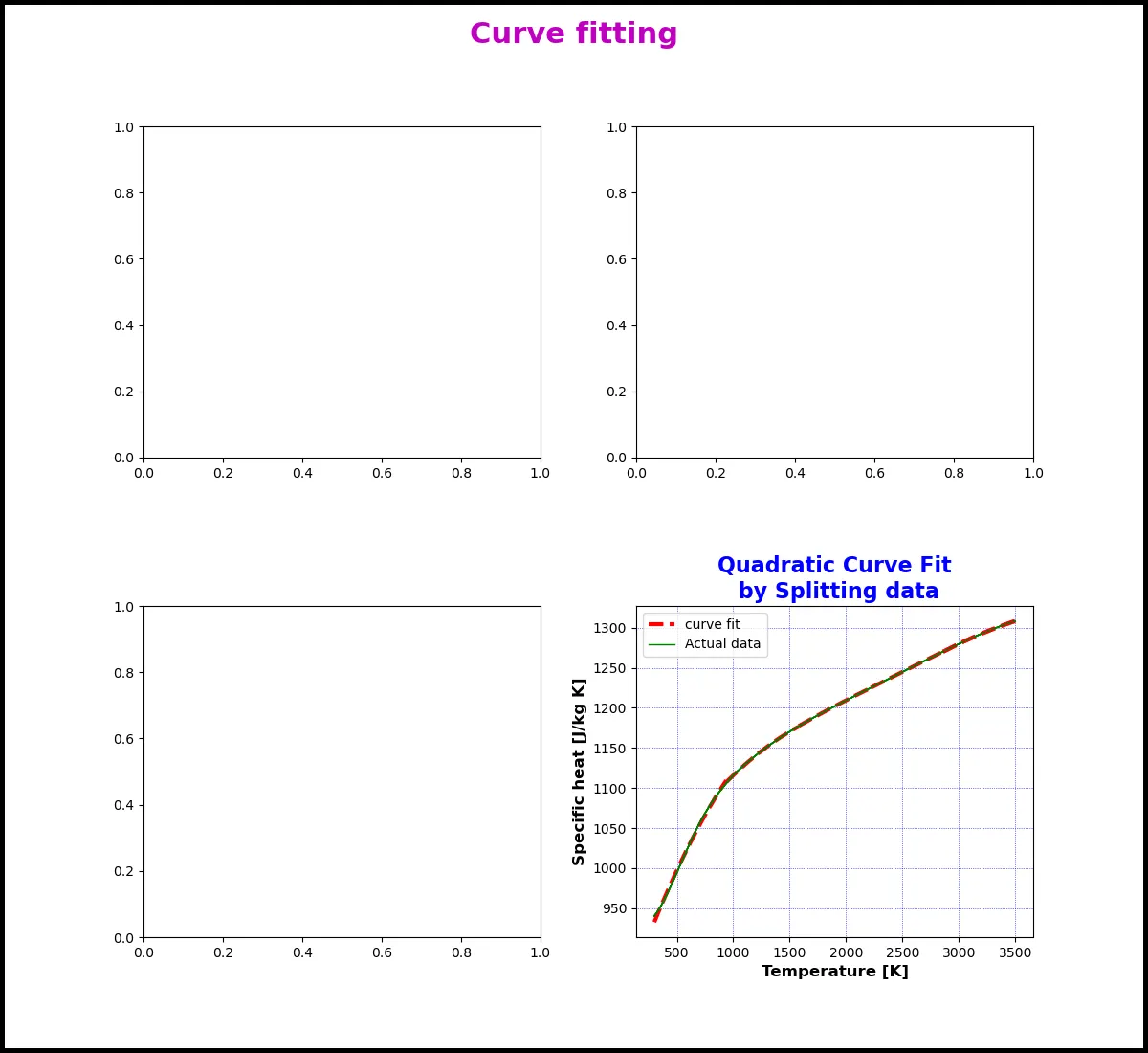
To improve curve fitting in more better way we can also split our data set into specific intervals and plot those intervals one accordingly. We create those intervals by dividing number of quantity into required intervals.

Here we have divided data into 5 intervals. And in a bid to plot in accordingly we are going to use for loop. By which we get stat and end value for each interval that range then we are going to assign to temperature data interval and cp data interval.

Furthermore, we are going to use quadratic curve fit for each interval, we can pic any polynomial function as per our need. And plot the result in graph.

The result will run for 5 intervals 5 time to plot he complete graph. Following are the codes to create intervals and to plot the graph.

and to plot the graph.
Fit_Interval = 5

for i in range(0,Fit_Interval+1):
	start = (3200/Fit_Interval)*(i-1)
	end = (3200/Fit_Interval)*i-1

	temperature_Int = temperature[int(start):int(end)]
	cp_Int = cp[int(start):int(end)]

	popt, pcov = curve_fit(Quadratic, temperature_Int, cp_Int)
	fit_cp_split = Quadratic(np.array(temperature_Int),*popt)

	ax4.plot(temperature_Int, fit_cp_split,'--', color='r',linewidth='3')
	ax4.plot(temperature, cp, color='g', linewidth='1')
	ax4.legend(['curve fit','Actual data'])
	ax4.set_title('Quadratic Curve Fit\n by Splitting data',color='b',size='16',weight='bold')
	ax4.set_xlabel('Temperature [K]',size='12',weight='bold')
	ax4.set_ylabel('Specific heat [J/kg K]',size='12',weight='bold')
	ax4.grid(color='b',linestyle=':',linewidth='0.5')

plt.savefig('Quadratic Curve Fit by Splitting data.png')

Output plot for above codes :-

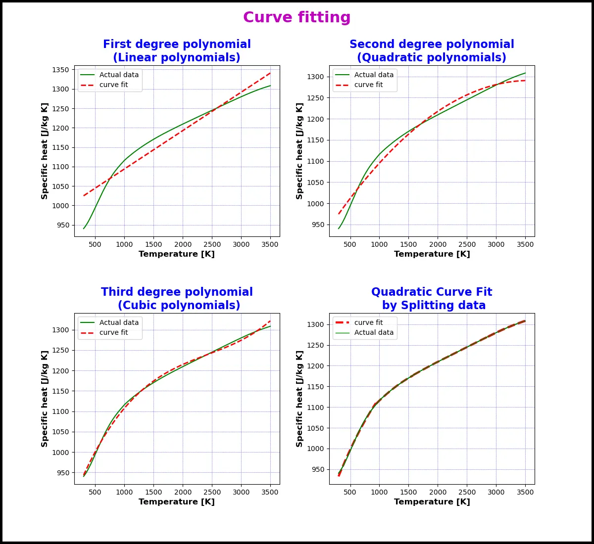
To compare all the curve fit in our final chart look will look like this.

plt.savefig('Curve fitting.png')

Final Output:-

Questions and answer

[1] What does popt and pcov mean?

popt (1-D array) - Optimal values for the parameters so that the sum of the squared residuals of f(xdata, *popt)-ydata in minimize.

Its decide the value of co-efficient for a polynomial taken for the approximation of the real data so that the ‘list square method’ of error regression estimation is satisfied.

Pcov(2-D array) - The estimated covariance of popt. The diagonals provide the variance of the parameter estimate.

In other words, pcov decides the covariance for the given optimum values for the curve, which in our case is coefficients of an approximation polynomial.

[2] What does np.array(temperature) do?

np.array(temperature) is the function in numpy library to feed the temperature array or data from the data file with their coefficient values to predict cp (Specific heat value) by passing those value through polynomial function or equation.

[3] What does the * in *popt mean?

Predicted_array by using function is calculated by using xdata and optimum value for the co-efficient of the equation. In this case, ‘*’ in ‘*popt’ is used to pass all the required positional arguments to determine function means pass all the coefficients value from function.

Predicted_y_array = func(np.array(xdata), *popt)

*popt feeds the value of the optimum coefficient obtained by the least squre method of error regression. Curve_fit function generates optimum parameter value for a given data set then stores it inside output called popt. Which is then use as a function handle for calculating predicted cp value.

[4] Write code to fit a linear and cubic polynomial fo the Cp data. Explain if your results are good or bad.

From above plot generated by python program we can say that the curve fit getting better as we are increasing the degree of polynomial in the equation and in order to reduce more errors in curve fit we can also split data in preferable interval which are giving better results.

[5] What needs to be done in order to make the curve fit perfect?

As we observe and study from above experiment we can minimize the error and curve fit variation by increasing the order of equation to n+1 degree polynomial.

Another method to get more better fit or minimum error is to divide the data into preferable intervals and then try to fit it with each interval of the main data as per our final plot in this experiment.

Conclusion-

• Observation based on output plots and figure, we get to know that, errors in the curve fit can be minimize by implementing higher degree polynomial.
• Second, method to reduce error in curve fitting is to splitting data in particular sets and then plot it by using preferable degree of polynomial.
• Finally, understood the implementation of scipy.optimize.curve_fit from scipy library

References:-

[1]scipy.optimize.curve_fit - https://docs.scipy.org/doc/scipy/reference/generated/scipy.optimize.curve_fit.html

[2]Gurley. Numerical Methods Lecture 5– Curve Fitting Techniques. CGN 3421 Lecture Notes. Retrieved from http://web.iitd.ac.in/~pmvs/courses/mel705/curvefitting.pdf

[3]Husch, Lawrence. Visual Calculus: Curve Fitting. Retrieved from http://archives.math.utk.edu/visual.calculus/0/curve_fit.5/index.html

Complete Program:-

import numpy as np 
import matplotlib.pyplot as plt
from scipy.optimize import curve_fit


# Curve fit function
# First degree polynomial (Linear polynomials)
def Linear(t,a,b):
	return a*t + b

# Second degree polynomial (Quadratic polynomials)
def Quadratic(t,a,b,c):
	return a*(t**2) + b*t + c

# Third degree polynomial (Cubic polynomials)
def Cubic(t,a,b,c,d):
	return a*(t**3) + b*(t**2) + c*t + d


# Reading thermodynamic data file
def read_file():
	temperature=[]
	cp = []
	for line in open('data','r'):
		values = line.split(',')
		temperature.append(float(values[0]))
		cp.append(float(values[1]))
	return [temperature, cp]



# Subplot for the figure1 and figure two
fig = plt.figure(figsize=(12,11),linewidth=6, edgecolor="k")
ax1 = plt.subplot2grid((12, 11), (0, 0), colspan=5,rowspan=5)
ax2 = plt.subplot2grid((12, 11), (0, 6), colspan=5,rowspan=5)
ax3 = plt.subplot2grid((12, 11), (7, 0), colspan=5,rowspan=5)
ax4 = plt.subplot2grid((12, 11), (7, 6), colspan=5,rowspan=5)
fig.suptitle('Curve fitting',size='22',weight='bold',color='m')


# Main program
temperature, cp = read_file()

popt, pcov = curve_fit(Linear, temperature, cp)
fit_cp_Linear = Linear(np.array(temperature), *popt)

ax1.plot(temperature, cp, color='g', linewidth='1.5')
ax1.plot(temperature, fit_cp_Linear,'--', color='r',linewidth='2')
ax1.legend(['Actual data','curve fit'])
ax1.set_title('First degree polynomial\n(Linear polynomials)',color='b',size='16',weight='bold')
ax1.set_xlabel('Temperature [K]',size='12',weight='bold')
ax1.set_ylabel('Specific heat [J/kg K]',size='12',weight='bold')
ax1.grid(color='b',linestyle=':',linewidth='0.5')



popt, pcov = curve_fit(Quadratic, temperature, cp)
fit_cp_Quadratic = Quadratic(np.array(temperature), *popt)

ax2.plot(temperature, cp, color='g', linewidth='1.5')
ax2.plot(temperature, fit_cp_Quadratic,'--', color='r',linewidth='2')
ax2.legend(['Actual data','curve fit'])
ax2.set_title('Second degree polynomial\n(Quadratic polynomials)',color='b',size='16',weight='bold')
ax2.set_xlabel('Temperature [K]',size='12',weight='bold')
ax2.set_ylabel('Specific heat [J/kg K]',size='12',weight='bold')
ax2.grid(color='b',linestyle=':',linewidth='0.5')



popt, pcov = curve_fit(Cubic, temperature, cp)
fit_cp_Cubic = Cubic(np.array(temperature), *popt)

ax3.plot(temperature, cp, color='g', linewidth='1.5')
ax3.plot(temperature, fit_cp_Cubic,'--', color='r',linewidth='2')
ax3.legend(['Actual data','curve fit'])
ax3.set_title('Third degree polynomial\n (Cubic polynomials)',color='b',size='16',weight='bold')
ax3.set_xlabel('Temperature [K]',size='12',weight='bold')
ax3.set_ylabel('Specific heat [J/kg K]',size='12',weight='bold')
ax3.grid(color='b',linestyle=':',linewidth='0.5')


Fit_Interval = 5

for i in range(0,Fit_Interval+1):
	start = (3200/Fit_Interval)*(i-1)
	end = (3200/Fit_Interval)*i-1

	temperature_Int = temperature[int(start):int(end)]
	cp_Int = cp[int(start):int(end)]


	popt, pcov = curve_fit(Quadratic, temperature_Int, cp_Int)
	fit_cp_split = Quadratic(np.array(temperature_Int),*popt)

	ax4.plot(temperature_Int, fit_cp_split,'--', color='r',linewidth='3')
	ax4.plot(temperature, cp, color='g', linewidth='1')
	ax4.legend(['curve fit','Actual data'])
	ax4.set_title('Quadratic Curve Fit\n by Splitting data',color='b',size='16',weight='bold')
	ax4.set_xlabel('Temperature [K]',size='12',weight='bold')
	ax4.set_ylabel('Specific heat [J/kg K]',size='12',weight='bold')
	ax4.grid(color='b',linestyle=':',linewidth='0.5')

plt.savefig('Curve fitting.png')
plt.show()

Final Output Plot:-