Week 5.2 - Literature review: ODE Stability

Abstract: Ordinary Differential Equation literature review.

Ordinary Differential Equation:

Ordinary differential equation (ODE) is a differential equation containing one or more functions of one independent variable and the derivatives of those functions.

Mathematical descriptions of change use differentials and derivatives. Various differentials, derivatives, and functions become related via equations, such that a differential equation is a result that describes dynamically changing phenomena, evolution, and variation.

Stability of an ODE:

When an ODE is solved numerically there accumulates an error which depends on the technique used to solve the equation and the time steps.

In our study we use the following equation

`dy/dt=-1000y-eoverset(-t)()`

The above equation is solved using Explicit and Implicit form

`yoverset(n+1)()= yoverset(n)()-dt(1000yoverset(n)()-eoverset(-t)())`=>Explicit

`yoverset(n)()= yoverset(n-1)()-dt(1000yoverset(n)()-eoverset(-t)())`=>Implicit

`yoverset(t)()= (eoverset(-1000t)()(1-eoverset(-999t)()))/999`=>Analytical

Below program used to compute the results for various time steps:

"""
ODE Stability
"""
import math
import numpy as np
import matplotlib.pyplot as plt

def explicit_euler(total_t, dt):
	t=np.arange(0,total_t,dt)
	y=np.zeros(len(t))

	for i in range(1, len(t)):
		y[i]=y[i-1]+dt*(-1000*y[i-1]-np.exp(-t[i-1]));

	return[t, y]

def implicit_euler(total_t, dt):
	t=np.arange(0,total_t,dt)
	y=np.zeros(len(t))

	for i in range(1, len(t)):

		y[i]=(y[i-1]-np.exp(-t[i-1])*dt)/(1+1000*dt)

	return[t,y]

def analytical(total_t, dt):
	t=np.arange(0,total_t,dt)
	y=np.zeros(len(t))

	for i in range(1,len(t)):
		y[i]=np.exp(-1000*t[i])*(1-np.exp(999*t[i]))/999
	return y

total_t=0.1
dt=1e-3
t, y_explicit=explicit_euler(total_t,dt)
t, y_implicit=implicit_euler(total_t,dt)
y_analytical=analytical(total_t,dt)
plt.plot(t,y_explicit,color='blue')
plt.plot(t,y_implicit,color='black')
plt.plot(t,y_analytical,color='orange')
plt.legend(['Explicit','Implicit','Analytical'])
plt.show()

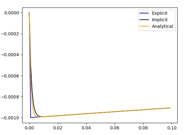
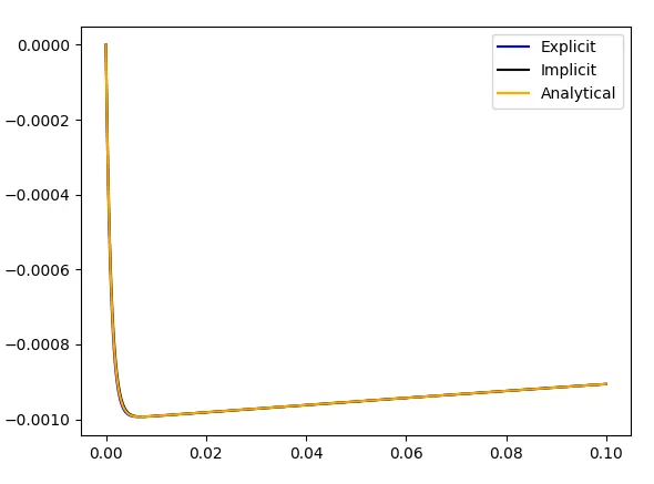
Plots for various time steps

Time step: 1e-3 Time step: 1e-4

Time step: 5e-3

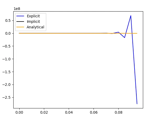
The above plots shows that by increasing timesteps gives unstable results.

When does an ODE becomes unstable?

We derive numerical approximations to solve an ODE, whenever this kind of numerical approximation is derived

it includes an error based on the order of approximation. If the derived numerical scheme is unstable then it starts

growing as time progresses.

In an explicit method when the timestep becomes more than the grid size there arises an unstability.

How does stability affects engineering simulations?

Unstable solutions end up incorrect results which will eventually reduce the authencity of the simulation.

It gives a unphysical result which we can't use for our study.

Can stability condition derive for all kinds of problem?

Stability condition is more accurate for linear systems. For non linear system, we need to perform linearization which is more of like an approximation eventually its results were not accurate.

1. Eigen value analysis

2. Von-neumann stability analysis

These are the two method we can used to determine the stability of the numerical scheme.