Week 5.2 - Literature review: ODE Stability

Aim:

To study stability of an ODE and its effect on engineering simulation.

AN ODE contains derivatives of one or more functions of an independent variable. To solve an ODE we need to determine the function or set of functions that satisfy the equation.

Al though many differential equations cannot be solved or are very lengthy and tedious to solve in case of the engineering simulations. Thus, for engineering applications numerical integration schemes are used for getting the approximation for the ODE’s. In case of time integrations these numerical integrations can be classified as explicit or implicit scheme. Euler method or forward differencing is the example of explicit scheme whereas backward differencing or backward Euler method is the example for the implicit scheme.

The numerical approximation for the ODE function is said to be stable if the solution of the equation remains close to each other for the exceed value of x. If the difference between the solutions approaches 0 with successive values of x then the solution is said to be asymptotically stable. If the solution remains stable for the arbitrarily large step sizes then the solution is called as unconditionally stable. If the solution doesn’t match either of the properties then the solution is called as unstable.

While using the explicit schemes some ODE’s can turn unstable and thus can be characterised as the stiff equations. Such kind of ODE’s cannot be solved using the explicit method until or unless the step size is taken too small. These kinds of ODE’s are generally stable with implicit technique but are not always unconditionally stable.

The stability of an ODE can be illustrated by calculating the analytical solution and approximation using explicit and implicit technique. The ODE used is :

`dy/dt = -1000y-e^(-t)`

The analytical solution of the solution can be written as:

`y(t) = frac{e^(-1000t)(1-e^(999t))}{999}`

The explicit solution of the solution can be written as:

`frac{y^(n+1)-y^n}{dt} = -1000y^n-e^-t`

`y^(n+1) = y^n-(1000y^n+e^-t)dt`

The implicit solution of the solution can be written as:

`frac{y^n - y^(n-1)}{dt} = -1000y^n-e^-t`

`y^n = frac{y^(n-1) - e^-tdt}{1+1000dt}`

Python Code

import matplotlib.pyplot as plt
import numpy as np
import math as mt

'''
ODE = dy/dt = -1000y-e^(-t)

Analytical Solution 
y(t) = (e^(-1000t)(1-e^(999t)))/999

Explicit Method
y^(n+1) = y^n - (1000y^n + e^(-t))dt

Implicit Method
y^(n) = (y^(n-1) - e^(-t))dt)/(1+1000dt)
'''
total_t = 0.1
dt = 1.9e-3
t = np.arange(0,total_t,dt)
y = np.zeros(len(t))

def analytical(total_t,t):
	t = np.arange(0,total_t,dt)
	y = np.zeros(len(t))
	for i in range(1,len(t)):
		y[i] = (mt.exp(-1000*t[i])*(1-mt.exp(999*t[i])))/999
	return[t,y]

def explicit(total_t,t):
	t = np.arange(0,total_t,dt)
	y = np.zeros(len(t))
	for i in range(1,len(t)):
		y[i] = y[i-1] - (1000*y[i-1] + mt.exp(-t[i-1]))*dt
	return[t,y]

def implicit(total_t,t):
	t = np.arange(0,total_t,dt)
	y = np.zeros(len(t))
	for i in range(1,len(t)):
		y[i] = (y[i-1] - (mt.exp(-t[i-1]))*dt)/(1+1000*dt)
	return(t,y)

t,y_explicit = explicit(total_t,t)
t,y_implicit = implicit(total_t,t)
t,y_analytical = analytical(total_t,t)
plt.plot(t,y_explicit,'b',label='Explicit')
plt.plot(t,y_implicit,'g',label='Implicit')
plt.plot(t,y_analytical,'r',label='Analytical')
plt.legend()
plt.show()

Plot

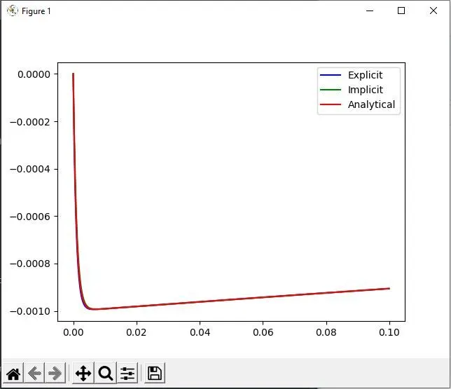
Step Size - 1.5e-4

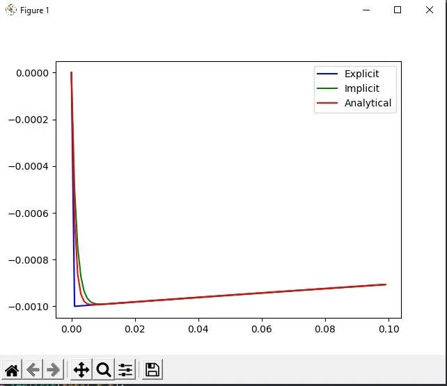
Step Size - 1e-3

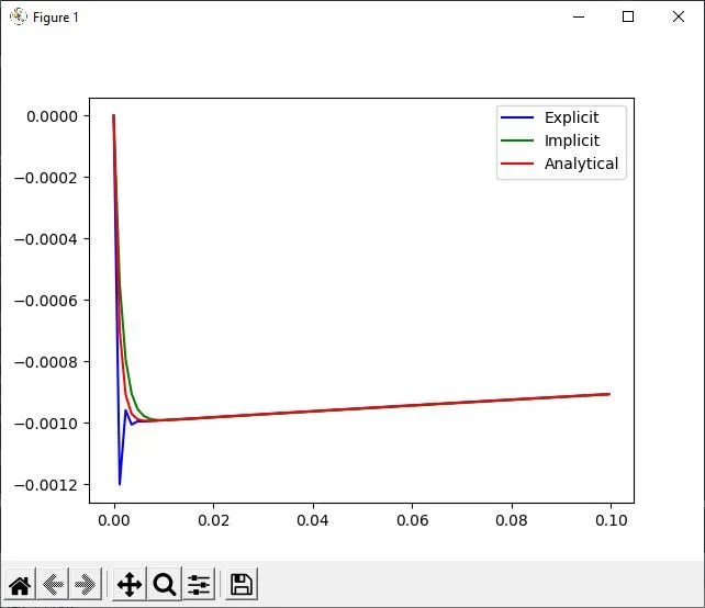
Step Size - 1.2e-3

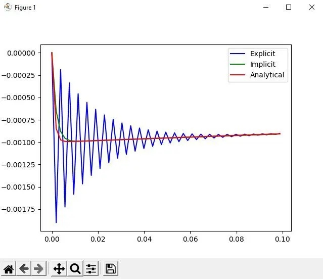
Step Size - 1.9e-3

Observation

The above four plots were taken with the successively increasing values of ‘dt’. It can be seen that as the time step size increased in the explicit solution, a small error generated and starts to amplify with successive increase in the step size. Whereas in the implicit solution a smooth plot can be seen as compared to analytical answer. Although some gap can be seen at certain areas of inflection which can be justified by numerical approximation.

Stability of an ODE is crucial to obtain the result in the engineering simulations as unstable ODE’s can give bogus results which are not relevant and thus should be discarded.

Every problem that needs to be solved is based on an expression. It is always important to know that expression is continuous in its inputs, which means that with the slight change in input will result in a slight change in output. If the expression gives large change in output with slight change in input than it can be considered as ill-conditioned. The exact cut-off between ill-conditioned and well-conditioned expression depends upon context of problem and use of the results.