Week 5.2 - Literature review: ODE Stability

When does a ODE become unstable?

When a solution to ordinary differential equation is approached by iterative numerical methods, the absolute error between iterations gives us an idea about the stability of the solution. For a stable solution, the error between the iterations should decrease. The step size in the iterative method along with the discrete point density in the domain of itegration plays a vital role in the stability of the upcoming solution.

Appropriate selection of step size and grid density is very vital for a stable solution.

How does stability affect engineering simulations?

If the solution to the differential equation has non stable characteristics, the gained values of variables might be unrealistic, there might be too much variation with the actual experimental results. Such solution are unacceptable and should not be trusted for further study.

There are various stability criterion developed for particular type of differential equations.

In order to demonstrate stability criterion, following stdy with a differential equation has been done.

Let us assume the differential equation to be:

`{dy}/{dt} = -1000y - e^{-t}`

Using explicit numerical method, solving the differential equation:

`{y_{"new"} - y_{"old"}}/{Deltat} = -1000y_{"old"} - e^{-t}`

Using Implicit numerical method, solving the differential equation:

`y_{"new"} = {y_{old} - e^{-t}Deltat}/{1+1000Deltat}`

Analytical Solution:

`e^{-1000t}*{1 - e^{999t}}/{999}` 

The code:-

import matplotlib.pyplot as plt
import numpy as np

# Solution by explicit method as discussed above
def explicit_euler(T,dt):
	t = np.arange(0,T,dt)
	y = np.zeros(len(t))
	

	for i in range(1,len(t)):
		y[i] = y[i - 1] + dt*( -1000*y[i - 1] - np.exp(-t[i - 1]))
	return [t,y]

# Solution by implicit method using backward difference approach as discussed above
def implicit_euler(T,dt):
	t = np.arange(0,T,dt)
	y = np.zeros(len(t))

	for i in range(1,len(t)):
		y[i] = (y[i - 1] - np.exp( -t[i - 1])*dt)/(1 + 1000*dt)

	return [t,y]

# Analytical solution of the given differential equation as discussed above
def analytical_euler(T,dt):
	t = np.arange(0,T,dt)
	y = np.zeros(len(t))

	for i in range(1,len(t)):
		y[i] = (np.exp( -1000*t[i])*(1 - np.exp((1000 - 1)*t[i])))/(1000 - 1)

	return [t,y]


# final t; T
T = 0.1
# Step Size
dt = 1.5e-3


dt_array = [0.01, 0.001, 0.0001, 0.00001]


for i in range(len(dt_array)):
    t,eqn_explicit = explicit_euler(T,dt_array[i])
    t,eqn_implicit = implicit_euler(T,dt_array[i])
    t,eqn_analytical = analytical_euler(T,dt_array[i])
    plt.figure(i+1)
    plt.plot(t,eqn_explicit,'--',color='red')
    plt.plot(t,eqn_implicit,'-.',color='blue')
    plt.plot(t,eqn_analytical,color='green')
    plt.xlabel('Time (t)')
    plt.ylabel('y')
    plt.legend(['Explicit-Solution','Implicit-Solution','Analytical-Solution'])
    plt.show(block=False)
    
plt.show()

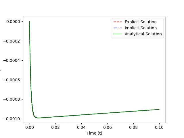
In the above program the time-step size has been been reduced by a factor of 10 in successive simulations. After we get the slution, the results from explicit, implicit as well as analytical solution has been compared.

dt = 0.01

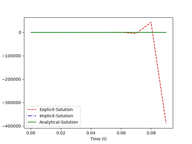
Unstable Explicit solution at dt = 0.01 (comparative large time step size)

dt = 0.001

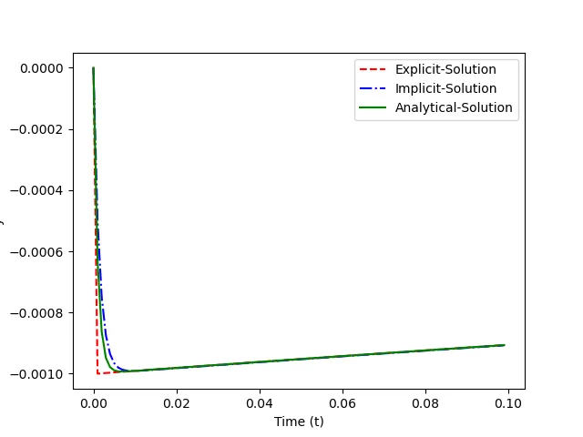
Under-estimated explicit solution and over-estimated implicit solution at some points with relatively smaller time step. It shows, the solution is stabilizing with reduced time step size.

dt = 0.0001

dt = 0.00001

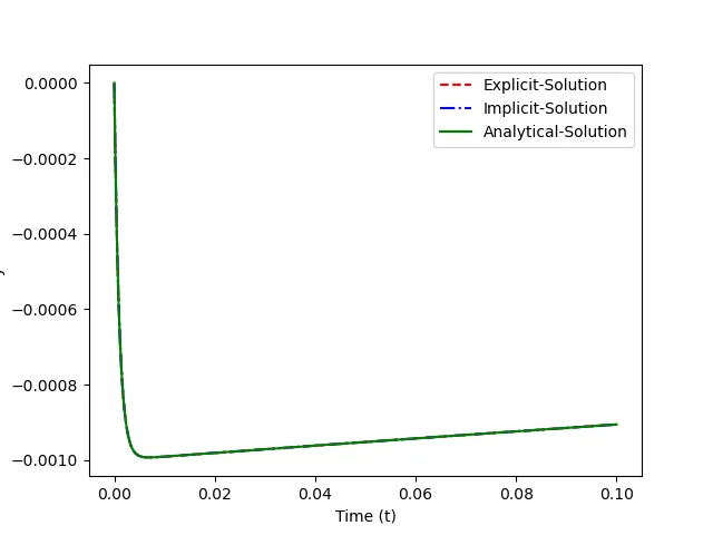
As can be seen from the above plots, the more we decrease the time step size, the more numerical solution shows similarity with the analytical solution.