Week 5.2 - Literature review: ODE Stability

Aim:

An ODE is an equation with a function in one independent variable as unknown, containing not only the unknown function itself, but also its derivatives of various orders. Ordinary differential equations (ODEs) arise in many contexts of mathematics and natural sciences. From electrical circuits to structural mechanics and modelling stock trends, ODE finds applications in all major scientific fields.

The generic way of representing an ODE is `y'(t) = f(t, y(t))` , for `y(t_0) = y_0`. --(1)

This ODE is IVP or initial value problem as along with the equation an initial condition is used to specify the initial condition.

Although, a simple ODE can be solved manually as the complexity of the ODE increases it becomes very difficult to obtain solution using analytical method. Hence, use of numerical integration methods are done to obtain the solution of such complex engineering problems.

Two such methods are discussed below:

• Explicit Method (Euler Method): The general approach of following using this method is as follows:

`y'(t) approx frac{y(t + h) - y(h)}{ h}`

`y(t + h) approx y(t) + h.y'(t)`

Using (1), we get

`y(t + h) approx y(t) + h.f(t, y(t))`

Now a step size, `h` is chosen and the above equation is solved in recursive way to obtain the solution. The generic form of explicit method can be expressed as : `y_(n+1) = y_n + h * f(t_n, y_n)`

However, one of the main disadvantages of the explicit method is that if the step size is too large convergence of solution becomes difficult, leading to formation of artificial errors. These artificial errors do not decay and rather increases every iteration due to which the scheme eventually fails to find a solution.

• Implicit Method (Backward Euler Method):

In case of implicit method, the approximation differs

`y'(t) approx frac{y(t) - y(t - h)}{ h}`

Solving this we get,

`y_(n+1) = y_n + h.f(t_(n+1), y_(n+1))`

The advantage of implicit method over explicit is that it is usually stable with large step sizes of stiff equations, however, implicit method is more computation intensive and hence takes requires more time to obtain the solution.

To demonstrate the working of both the methods a sample python code is written to solve the below ODE using both implicit, explicit methods. Along with numerical integration analytical method is also implemented to compare the differences.

ODE `f(t) = frac{dy}{dt} = -1000y - exp(-t)` for `y(0) = 0`

Coding Approach:

Three functions are written to calculate the solution for equation using analytical, implicit and explicit method. Each of these functions takes total time and time step as inputs.

The solution of the ODE is calculated using different time steps to observe its effect on solution. For all the cases of time steps a plot is generated for solution against the time.

Code:

import numpy as np
import matplotlib.pyplot as plt


def analytical_solution(total_t, dt):
    time_series = np.arange(0, total_t, dt)
    y = np.zeros(len(time_series))

    for i in range(1, len(time_series)):
        y[i] = (np.exp(-1000 * time_series[i - 1]) * (1 - np.exp(999 * time_series[i - 1]))) / 999

    return [time_series, y]


def explicit_euler(total_t, dt):
    time_series = np.arange(0, total_t, dt)
    y = np.zeros(len(time_series))

    for i in range(1, len(time_series)):
        y[i] = y[i - 1] - 1000 * y[i - 1] * dt - np.exp(-time_series[i - 1]) * dt
    return [time_series, y]


def implicit_euler(total_t, dt):
    time_series = np.arange(0, total_t, dt)
    y = np.zeros(len(time_series))

    for i in range(1, len(time_series)):
        y[i] = (y[i - 1] - np.exp(-time_series[i - 1]) * dt) / (1 + 1000 * dt)
    return [time_series, y]


total_time = 0.1
deltas = [0.09, 0.0018, 0.001, 0.0001]
total_plots = len(deltas)
for s_no, delta_t in enumerate(deltas):
    s_no += 1
    # plt.subplot(1, total_plots, s_no)
    plt.figure()
    time_explicit, y_explicit = explicit_euler(total_time, delta_t)
    time_implicit, y_implicit = implicit_euler(total_time, delta_t)
    time_analytical, y_analytical = analytical_solution(total_time, delta_t)

    plt.plot(time_explicit, y_explicit, time_implicit, y_implicit, "g--", time_analytical, y_analytical, "r--")
    plt.xlabel("Time")
    plt.ylabel("Solution (y)")
    plt.legend(["Explicit Euler", "Implicit Backward", "Analytical Solution"])
    plt.title(f"Time Step = {delta_t}")
    plt.tight_layout()
    plt.savefig(f"ODEStability_{delta_t}.png", dpi=300)

Results:

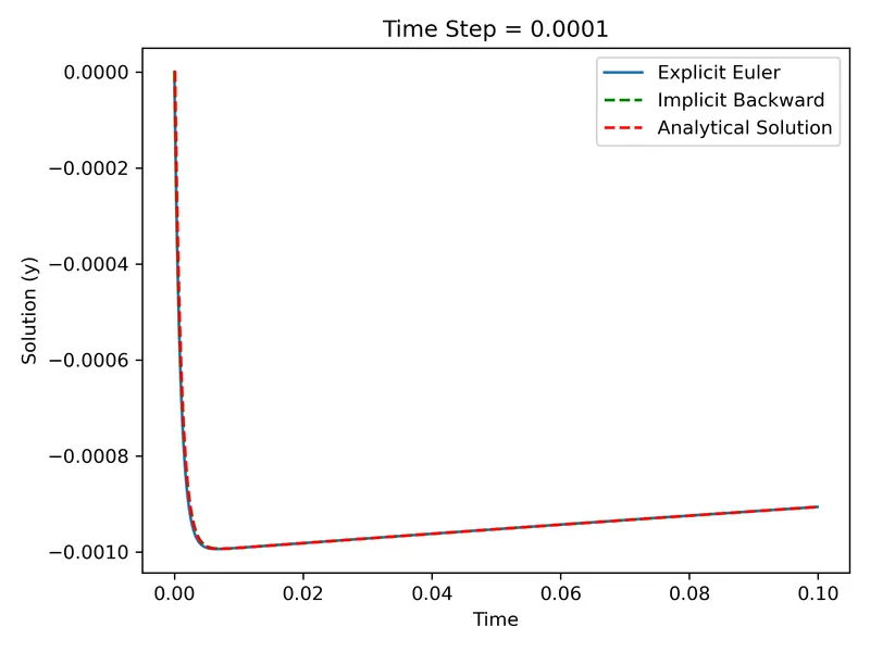
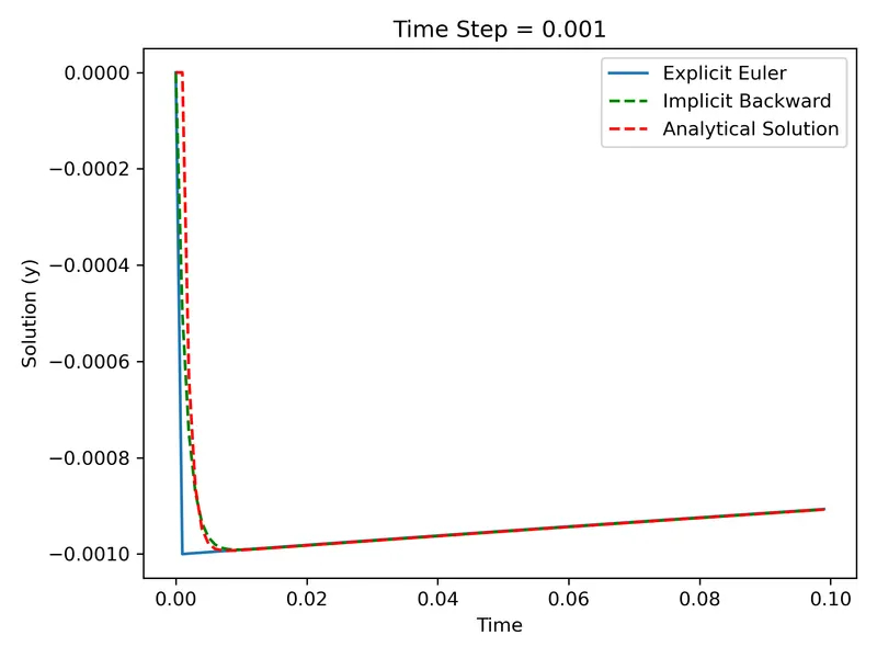
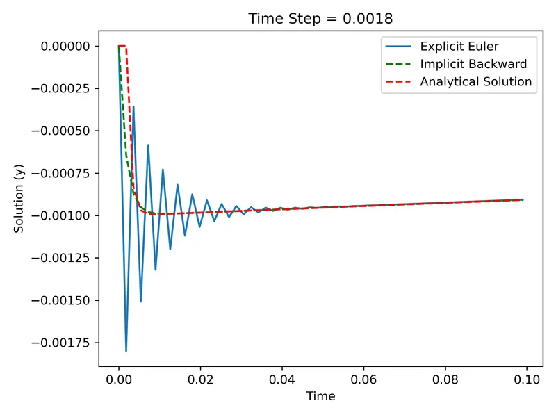
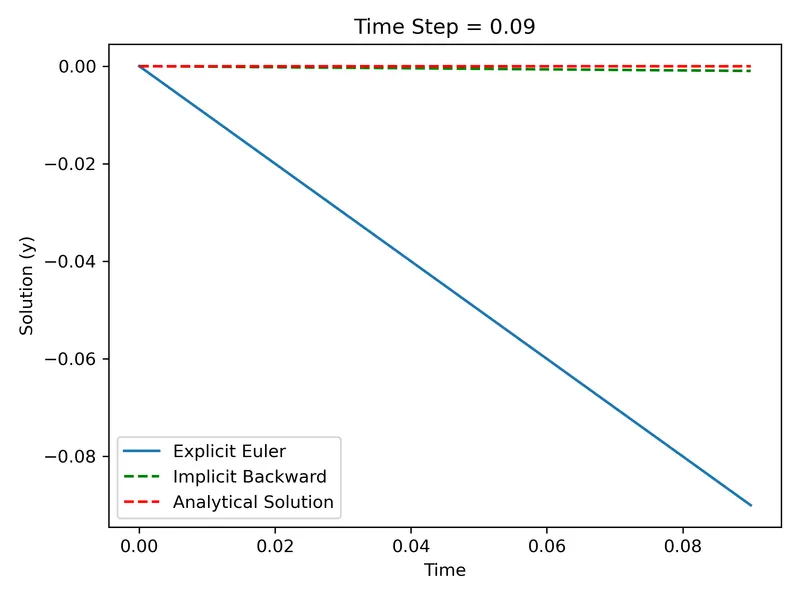
• From the graphs it can be observed that for higher time step(time step=0.09), explicit methods fails to obtain any solution, while for a lowest time step (time step = 0.0001) the solution matches with analytical as well implicit solution.
• Implicit solution is stable irrespective of time step size.
• In case of time step = 0.0018 aritificial errors are observed in case of explicit methods, which finally dissipates.
• As the time step is reduced the error between implicit solution and explicit solution also reduces.
• This shows that how a small change in one value can lead to unstable system and ultimately unstable solution. Owing to this, engineering systems needs to be carefully modelled to accomodate these perturbations.
• Stability of linear ODE can be calculated using Eigen values and Eigen Vectors, however, the approximations from these method are poor on a non-linear model.