Week 5.2 - Literature review: ODE Stability

AIM: To review the lieterature about Ordinary Differential Equation and to write the Python program on Stability. 

Theoritical Background:

Ordinary Differential Equation

The differential equation containing one or more functions of an independent variable and derivatives of those functions. But in the case ODE, the word ordinary is used for derivative of the functions for the single independent variable.

In mathematics, the term “Ordinary Differential Equations” also known as ODE is an equation that contains only one independent variable and one or more of its derivatives with respect to the variable. In other words, the ODE is represented as the relation having one independent variable x, the real dependent variable y, with some of its derivatives.

y’,y”, ….yⁿ ,…with respect to x

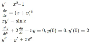
Examples of ODE

Applications of ODE

1] Modelling the growth of diseases

2] Describes the movement of electricity

3] Describes the motion of the pendulum, waves

4] Used in Newton’s second law of motion and Law of cooling

Stability of Ordinary Differential Equation(ODE)

In terms of the solution of a differential equation, a function f(x) is said to be stable if any other solution of the equation that starts out sufficiently close to it when x = 0 remains close to it for succeeding values of x. By using the numerical schemes in the computer we are going to solve ODE. These solutions schemes can be Implicit or Explicit. 

The general form of ODE is 

Consider the function which varies along time 't'

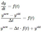
Implict Formulation

Explicit Formulation

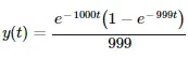
Analytical Expression

Explicit method

Explicit schemes lead at best to conditional stability. Conditional stability puts a limit on the timestep. We cannot progress too rapidly in time with the numerical scheme - as it may not be able to trasmit the information in the solution

Implicit method

Implicit schemes are generally unconditionally stable. Implicit methods have no such restriction on time step, but require more computation per timestep

PYTHON CODE:

import numpy as np
import matplotlib.pyplot as plt 

def explicit(t_total,dt):
	t=np.arange(0,t_total,dt) 
	y=np.zeros(len(t))

	for i in range(0,len(t)):

		y[i]=y[i-1]+dt*(-1000*y[i-1] -np.exp(-t[i-1]));
	return[t,y]	

def implicit(t_total,dt):
	t=np.arange(0,t_total,dt)
	y=np.zeros(len(t))

	for i in range(0,len(t)):
		y[i]=(y[i-1]-np.exp(-t[i-1])*dt)/(1+1000*dt);
	return[t,y]	

t_total=0.1
dt=0.001
	
t,y_exp=explicit(t_total,dt)
t,y_imp=implicit(t_total,dt)

plt.plot(t,y_exp)
plt.plot(t,y_imp)

plt.legend(('Explicit','Implicit'))
plt.grid(True)
plt.show()	

PLOTS:

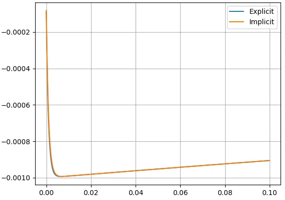
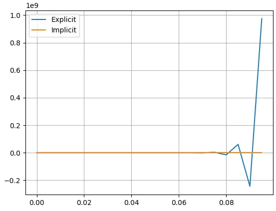
For the time step, dt = 0.0005                                                                       For the time step, dt = 0.0001

        

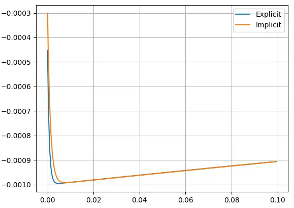
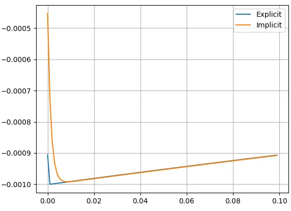
For the time step, dt = 0.005                                                                            For the time step, dt = 0.001

              

For the time step, dt = 0.002

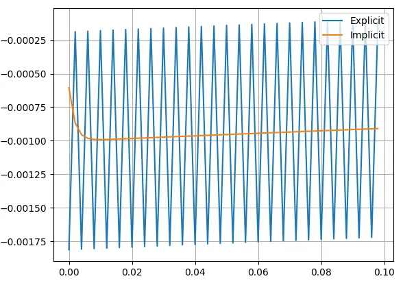
When we increase the number of grid points the simulation is going to slower because we are solving more equations When we are trying to run with large number of grid points the simulation is going to run really slow not because of increase number of grid points but also because of stability criterion and decrease in time step. From the above plot it can be observed that Implicit method gives stable soluton at higher value of 'dt'. The Time step plays a crucial role in determining the stability of the solution while using explicit method. 

When does a ODE become unstable?

Error in the solution is proportional to ‘delta t’. Larger the value of delta t, larger is the number of grid points and larger is the error. When there is more number of species and reactions we cannot calculate analytical expression easily, in that case Implicit method is the only way to obtain solution. At higher values of time step the solution starts to blow up, that is becoming unstable for explict method but remains stable for Implicit method.

How does stability affect engineering simulations?

If the solution becomes unstable the required value will deviate instead of converging. Stability gurantees that numerical solution produces bounded results. If the solution is not bounded the results starts to diverge and we don't get the proper output.

Can stability condition be derived for all types of problems?

Stability of the solution can be determined by below 2 ways

1] Eigen value analysis: Real Eigen values less than or equal to zero

2] Von-Neumann stability analysis: This can be applied when domain of the solution is periodic.