Week 5.2 - Literature review: ODE Stability

Literature review: ODE Stability

• Aim :

1. To do a literature review of ODE stability.
2. To answer the questions based on literature review.

Questions:

1. When does a ODE become unstable?
2. How does stability affect engineering simulations?
3. Can stability condition be derived for all types of problems?

• Introduction :

ODE - In mathematics, an ordinary differential equation (ODE) is a differential equation containing one or more functions of one independent variable and the derivatives of those functions. The term ordinary is used in contrast with the term partial differential equation which may be with respect to more than one independent variable.

Stability - In mathematics, condition in which a slight disturbance in a system does not produce too disrupting an effect on that system. In terms of the solution of a differential equation, a function f(x) is said to be stable if any other solution of the equation that starts out sufficiently close to it when x = 0 remains close to it for succeeding values of x. If the difference between the solutions approaches zero as x increases, the solution is called asymptotically stable. If a solution does not have either of these properties, it is called unstable.

To solve an ODE numerically there are two methods, namely explicit and implicit.

To understand how explicit and implicit methods work, let us consider an ODE

`dy/dt = -1000.y - e^(-t)`

where, y = molar concentration of a species

`dy/dt` = rate of change of molar concentration the species

1. Explicit Method : Explicit method is also known as forward differencing method. After discretizing we get,

`(y^(n+1) - y^n)/ dt = -1000.y^n - e^(-t)`

where, `y^n` = value of y at current time step

`y^(n+1)` = value of y at next time step

`y^(n+1) = y^n - 1000.y^n.dt - e^(-t).dt`

`y^(n+1) = y^n (1 - 1000.dt) - e^(-t).dt`

2. Implicit Method : Implicit method is also known as backward differencing method. After discretizing we get,

`(y^n - y^(n-1))/ dt = -1000.y^(n) - e^(-t)`

where, `y^n` = value of y at current time step

`y^(n-1)` = value of y at previous time step

`y^n - y^(n-1) = -1000.y^(n).dt - e^(-t).dt `

`y^(n-1) = y^n + 1000.y^n.dt + e^(-t).dt`

`y^(n-1) = y^n(1 + 1000.dt) + e^(-)t.dt`

`y^n = (y^(n-1) - e^(-t).dt)/ (1 + 1000.dt)`

Analytical solution : The ODE can be solved numerically. In this case we use Wolframalpha.com to get the solution for our ODE.

`dy/dt = -1000.y - e^(-t)`

`y(t) = e^(-1000.t).(1 - e^(999.t))/999`

Now, using python code to verify solution schemes,

import numpy as np
import matplotlib.pyplot as plt

def explicit(t_total,dt):
	t=np.arange(0,t_total,dt)
	y=np.zeros(len(t))


	for i in range(1,len(t)):
		y[i] = y[i-1] + dt*(-c*y[i-1] - np.exp(t[i-1]))
	return [t,y]

def implicit(t_total,dt):
	t=np.arange(0,t_total,dt)
	y = np.zeros(len(t))

	for i in range(1,len(t)):
		y[i] = (y[i-1]-np.exp(-t[i-1])*dt)/(1+c*dt)
	return [t,y]
	
def analytical(t_total,dt):
	t = np.arange(0,t_total,dt)
	y = np.zeros(len(t))

	for i in range(1,len(t)):
		y[i] = (np.exp(-c*t[i])*(1-np.exp((c-1)*t[i])))/(c-1)

	return [t,y]

t_total = 0.1
c = 1000
dt = 1e-5


t,y_explicit = explicit(t_total,dt)
t,y_implicit = implicit(t_total,dt)
t,y_analytical = analytical(t_total,dt)

plt.plot(t,y_explicit,'--', color = 'blue')
plt.plot(t,y_implicit, color = 'red')
plt.plot(t,y_analytical,'--', color = 'orange')
plt.xlabel('time')
plt.ylabel('y')
plt.legend(['Explicit','Implicit','Analytical'])
plt.show()

Plots -

Plots -

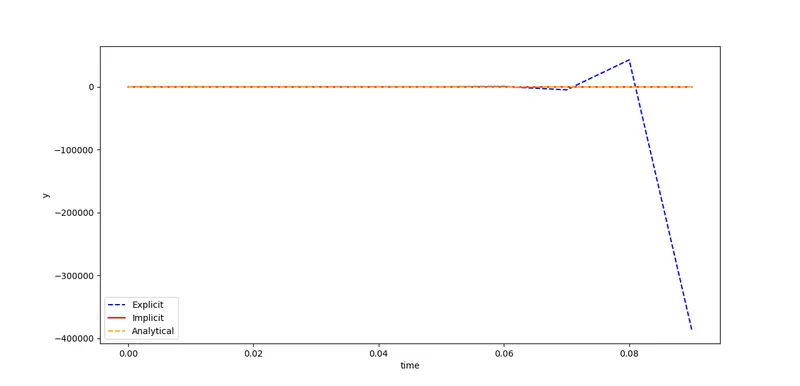
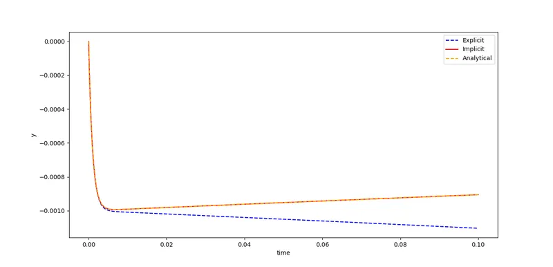
1. dt = 1e-2

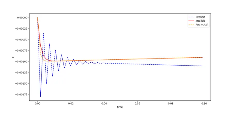
2. dt = 1.8e-3

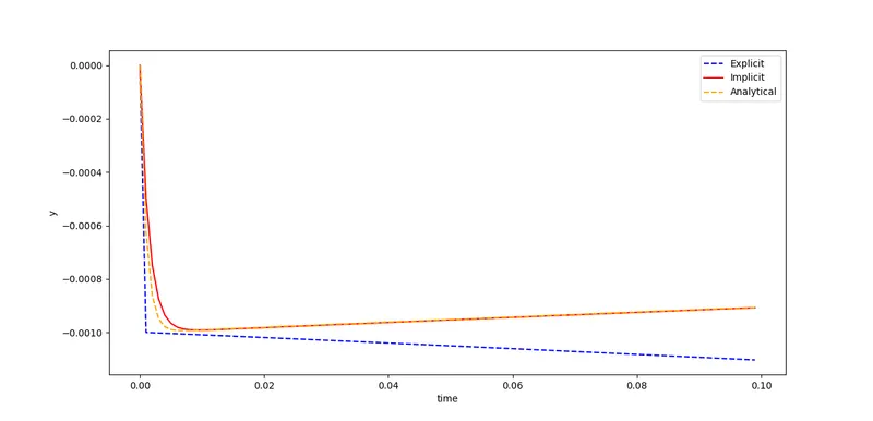
3. dt = 1e-3

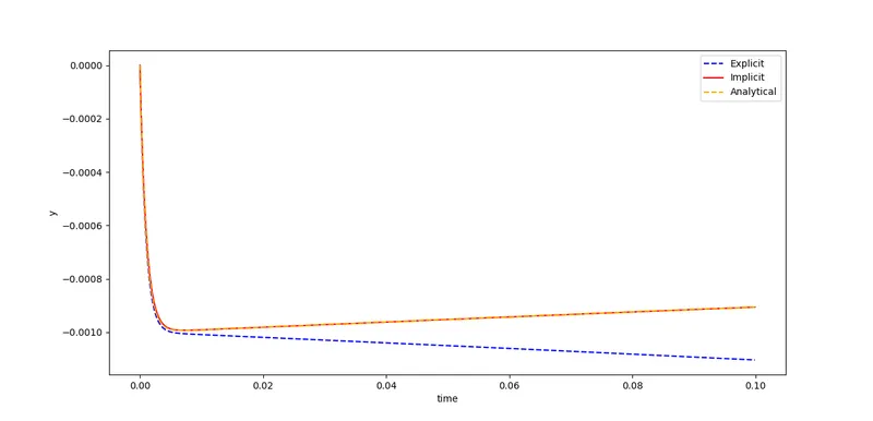
4. dt = 1e-4

5. dt = 1e-5

Q1. When does a ODE become unstable?

Ans : From the above plots we can concure that stability of ODE is dependant on value of dt.

In a general ODE, `dy/dt = y.lambda` , where `lamda` is coefficient of function

the ODE becomes stable if `|1+dt.lambda|le1` condition is met.

So if `lamda` increases we need to decrease the value of dt.

So for a solution to be stable, `dt le-2/(lambda)` condition needs to be satisfied.

Q2. How does stability affect engineering simulations?

Ans : Unstable solutions are obtained when big fluctuations or changes in solution are observed. These fluctuations are caused by errors and if these errors keep growing then the solution isn't going to be accurate. Thus, minimizing errors and finding accurate solutions is main aim of engineering simulations, so stability is very important.

Q. Can stability condition be derived for all types of problems?

Ans : Stability condition can be derived for linear ODEs only. For non linear ODEs stability can be predicted by forming a jacobian matrix and calculating eigen values. The solution is said to be stable if all eigen values are negative. The solution is said to be unstable if any one of the eigen values is positive.