Week 5.2 - Literature review: ODE Stability

Objective: To review the literature about ODE and to write the python program to substantiate our results.

When does an ODE become unstable?

When we writing code for explicit form solution goes unstable because if the time step is really large, nos. of grid points really large, convective velocity really large.
Numerical stability has to do with the behavior of the solution as the time-step 'dt' is increased. If the solution remains well behaved for arbitrarily large values of the time step, the method is said to be unconditionally stable. This situation never occurs with explicit methods, which are always conditionally stable. It is easy to see that this is so by dividing the
Y-equation by 'dt' and then letting 'dt' approach infinity. In this limit there are no n+1 terms remaining in the equation so no solution exists for yⁿ⁺¹, indicating that there must be some limit on the size of the time step for there to be a solution.

How does stability affect engineering simulations?

It is always bad to have an unstable solution for any kind of engineering simulation because it gives us un-physical results.
e.g. If we are running the simulation of aerofoil and we got the unstable solution then the drag coefficient and lift coefficient we are calculating will be unphysical and we can not trust this simulation.

Can stability conditions be derived for all types of problems?

There are two ways to determine or derive the stability of problems-
1. Eigen Value analysis- Real eigenvalues less than or equal to Zero
2. Von-Neumann stability analysis- This can be applied when solution domain is periodic.

An ordinary differential equation (ODE) is an equation that involves some ordinary derivatives (as opposed to partial derivatives) of a function. Often, our goal is to solve an ODE, i.e., determine what function or functions satisfy the equation. It is also an equation that determines the relationship between function and one or more derivatives of that function.

For example, this is a differential equation that relates the function y(t) with its first and second derivatives:

`d^2/dt^2y(t)+1/4d/dty(t)+y(t)= sin(t)`

The above example is the Ordinary Differential Equation (ODE) because the unknown function y(t), is a function of a single variable, in this case, it is 't'. Because we are dealing with the function of a single variable, the only ordinary derivative of the function will appear in the equation.
If we are dealing with the function of two or more variables, the partial derivatives of the function would appear in the equation, and we would call this differential equation a Partial Differential Equation (PDE).

For example, the PDE is:

`(d^2u)/dx^2+(d^2v)/dy^2+(d^2w)/dz^2= c^2(d^2u)/dt^2`

Why do we required to study differential equatioins?
The reason is the differential equation arises is the mathematical model that describes the most physical process, for example, convection, turbulence, combustion, spray transfer, other physical phenomenons.

To solve the differential equation means to find a function that satisfies the equation.

Stability of ODE:

Stability of a particular solution of interest (eg a traveling wave or another type of coherent structure or pattern) means, roughly speaking, that if the system starts with an initial condition near that particular solution, then the system will stay near it for all time.

All these ODE's, PDE's we are going to solve numerically with the aid of numerical schemes in computers. Numerical solution schemes are often referred to as being explicit or implicit. When a direct computation of the dependent variables can be made in terms of known quantities, the computation is said to be explicit. In contrast, when the dependent variables are defined by coupled sets of equations, and either a matrix or iterative technique is needed to obtain the solution, the numerical method is said to be implicit.

The general form of ODE is:

Let us consider any function which varies along with time 't'.

`dy/dt=f(t)`

`(y^("new")-y^("old"))/(Deltat)=f(t)`

`y^("new")=Deltat*f(t)+y^("old")`

Rewritting above equation as:

`y^("new")=y^("old")+Deltat*f(t)`

`y^("n+1")=y^("n")+dt*f(t)`

For example,

`dy/dt=-1000y - e^-t`

Explicite Formulation:

`y^("n+1")=y^("n")-dt*(1000y^n+e^-t)`

Implicite Formulation:

`y^("n")=y^("n-1")-dt*(1000y^n+e^-t)`

Analytical expression:

`y(t)=(e^(-1000t)(1-e^(-999t)))/999`

Python Code:

In this we are going to look at the effect of time step on solution. Time step we are going to cinsider is 1e-4, 5e-4, 10e-4, 15e-4, 20e-4.

import numpy as np
import matplotlib.pyplot as plt

dt= 1e-4; 
#To define the time step.
t_end= 0.1;

def explicit_euler(t_end, dt):

	t = np.arange(0,t_end,dt)
	y= np.zeros(len(t))

	for i in range (1,len(t)):
		y[i] = y[i-1] + dt * (-1000 * y[i-1] - np.exp(-t[i-1]));
	return [t,y]

def implicite_euler(t_end, dt):

	t = np.arange(0,t_end,dt)
	y= np.zeros(len(t))

	for i in range (1,len(t)):
		y[i] = (y[i-1] - np.exp(-t[i-1])* dt)/(1+1000*dt);

	return [t,y]

def analytical_solution(t_end, dt):

	t = np.arange(0,t_end,dt)
	y= np.zeros(len(t))

	for i in range (1,len(t)):
		y[i] = (np.exp(-1000*t[i-1])*(1-np.exp(999*t[i-1])))/999

	return [t,y]

t,y_e = explicit_euler(t_end,dt)
t,y_i = implicite_euler(t_end,dt)
t,y_ana = analytical_solution(t_end,dt)
plt.plot(t,y_e)
plt.plot(t,y_i)
plt.plot(t,y_ana,'--',color='black')
plt.legend(['explicit','implicite','analytical'])
plt.show()

Results:

The below graphs are showing a comparison of the stability of the solution for different time steps.

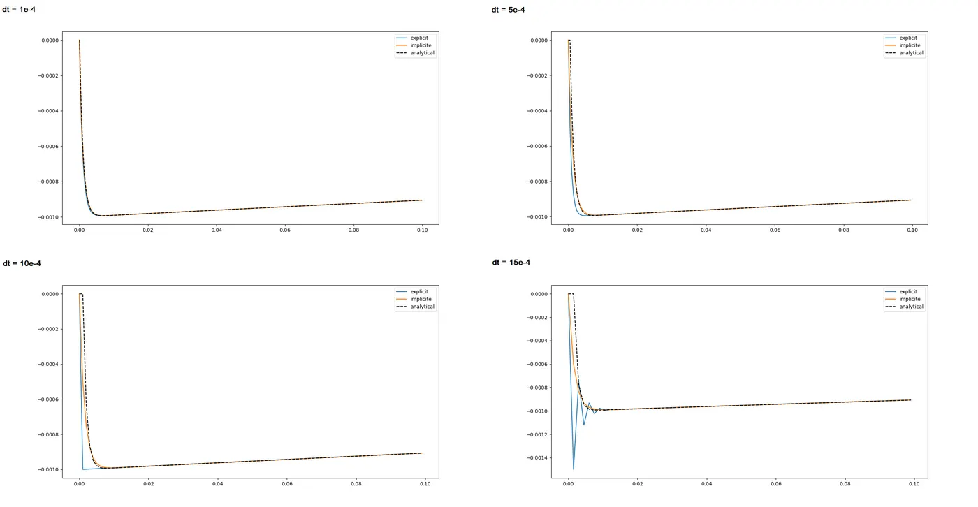
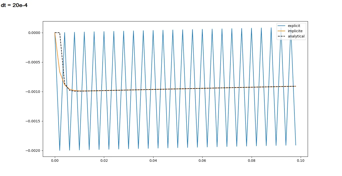
The graph clearly inferred that increase in timestep would cause instability in the final solution.