Week 5.1 - Mid term project - Solving the steady and unsteady 2D heat conduction problem
Problem Statement: Steady and Unsteady 2D heat conduction problem
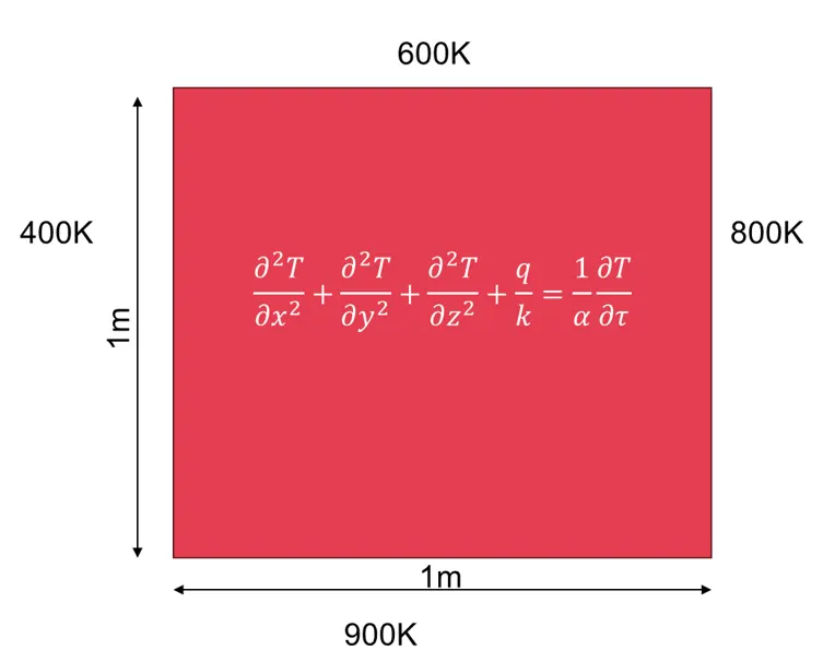
1.1 Objective: To write a MATLAB function for Steady state analysis and transient State Analysis. To Solve the 2D heat conduction equation by using the point iterative techniques that were taught in the class. The Boundary conditions for the problem are as follows.
a) Top Boundary = 600 K
b) Bottom Boundary = 900 K
c) Left Boundary = 400 K
d) Right Boundary = 800 K
You will implement the following methods for solving implicit equations.
· Jacobi
· Gauss-seidel
· Successive over-relaxation
a) Your absolute error criteria is 1e-4
- You will write code for both implicit and explicit schemes (This is for the transient analysis only)
- Compare the convergence rate [Number of iterations] of the steady state and transient [explicit and implicit] simulations and justify the numerics.
1.2 Theory:
The generalized 2D-Heat conduction PDE equation is given as follows.
`(∂^2 T)/(∂x^2 )+(∂^2 T)/(∂y^2 )+(∂^2 T)/(∂z^2 )+q/k=1/α (∂T)/(∂τ)…….(1)`
Where, T= temperature at nodes
q= Heat source generation
`alpha`= thermal diffusivity
A material's thermal diffusivity, a thermophysical attribute, is determined by dividing its thermal conductivity by its thermal capacity. Since there’s no heat source in the given problem we can neglect the heat generation part and nodes in z-coordinates. Therefore, the equation reflects the parabolic, unstable 2D heat conduction as follows,
`(∂^2 T)/(∂x^2 )+(∂^2 T)/(∂y^2 )=1/α ( ∂T)/(∂τ)…….(2)`
For, the steady state the time-derivative term can also be neglected hence making it an elliptic Laplace equation form,
`(∂^2 T)/(∂x^2 )+(∂^2 T)/(∂y^2 )=0…….…….(3)`
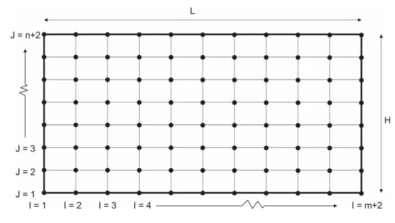
The discretization of the domain is done by the following method. The domain has been discretized into the grid. The discretized domain is presented in Figure below. Here the L=H=1m
m= Total number of vertical lines inside the domain
n= Total number of horizontal lines inside the domain
i= It is the ith vertical line
j= It is the jth horizontal line
m+2= The total number of vertical lines
n+2=The total number of horizontal lines
The given boundary conditions are:
To solve the equations numerically they are discretized as below,
- For the steady state 2D heat conduction,
`T_p=1/K [((T_r+T_l)/(∆x^2 ))+((T_t+T_b)/(∆y^2 ))]`
`where,K=2((∆x^2+∆y^2)/(∆x^2 ∆y^2 ))`
- The transient 2D heat conduction equation for the explicit method can be written as,
- `T_p^(n+1)=T_p^n+K_1 (T_r^n-2T_p^n+T_l^n )+K_2 (T_t^n-2T_p^n+T_b^n) where, K_1=α(∆t)/(∆x^2 ) and K_2=α(∆t)/(∆y^2 )`
The transient 2D heat conduction equation for the implicit method can be written as,
`T_p^(n+1)=1/((1+2K_1+2K_2))*[T_p^n+K_1 (T_r^n-2T_p^n+T_l^n )+K_2 (T_t^n-2T_p^n+T_b^n)]`
`where, K_1=α(∆t)/(∆x^2 )` and `K_2=α(∆t)/(∆y^2 )`
MATLAB CODE
The MATLAB code for the 2D steady state is written as follows:
1) The inputs like the length of domain, and boundary conditions are provided.
2) Making 3 separate loops for each scheme Jacobi, Gauss Siedel, and SOR schemes and asking the user to select the scheme required which then based on the input selects the desired method loop and solves for the 2D heat numerical equation.
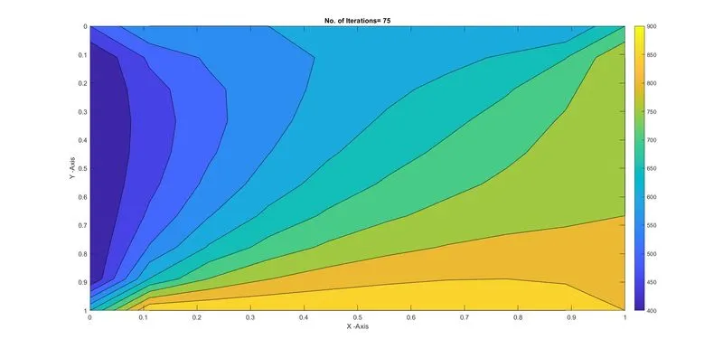
3) The number of iterations required is also displayed along with the contours of the heat conduction.
clear all
close all
clc

% Solving Steady state 2D heat conduction equation
% defining domain and nodes
n_nodes = 10;
length = 1; % domain length 1m

% value of x and y at nodes in a discretization plane
x = linspace(0,length,n_nodes);
y = linspace(0,length,n_nodes);
dx = length/(n_nodes-1);
dy = length/(n_nodes-1);


% let the initial temperture guess at all nodes be 300k
T = 300*ones(n_nodes,n_nodes);

% boundary conditions at left and right nodes
T(1:end,1) = 400;
T(1:end,end) = 800;

% boundary conditions at bottom and top nodes
T(end,1:end) = 900;
T(1,1:end) = 600;

% Average value of T at corners
T(1,1) = 500;
T(end,1) = 650;
T(1,end) = 700;
T(end,end) = 850;

% Storing the value of T
T_old = T;

%constant K and omega
K = (2*(dx^2+dy^2))/(dx^2*dy^2);
omega= 1.2;

% Convergence criteria
error = 10;
tol = 1e-4;
iter = 0;

% taking input for the type of iterative methods
method = input('Select 1 for Jacobi, Select 2 for Gauss siediel, Select 3  for Succesive Over-Relaxation (SOR) : ');
if method == 1 % For jacobi method
    while(error>tol)
        for i = 2:n_nodes-1
            for j = 2:n_nodes-1
            term1 = (T_old(i+1,j)+T_old(i-1,j))/dx^2;
            term2 = (T_old(i,j+1)+T_old(i,j-1))/dy^2;
            T(i,j) = (term1+term2)/K;
            end
        end
        error = max(max(abs(T_old-T)));

        % % to upadte the old velocity with the new one

        T_old = T;
        iter = iter+1;
    end
    disp('The total iterations for Jacobi method are')
elseif method == 2 % For Gauss Siedel method
    while(error>tol)
        for i = 2:n_nodes-1
            for j = 2:n_nodes-1
            term1 = (T_old(i+1,j)+T(i-1,j))/dx^2;
            term2 = (T_old(i,j+1)+T(i,j-1))/dy^2;
            T(i,j) = (term1+term2)/K;
            end
        end
        error = max(max(abs(T_old-T)));

        % % to upadte the old velocity with the new one

        T_old = T;
        iter = iter+1;
    end
    disp('The total iterations for Gauss-seidel method are')
else
    while(error>tol) % For SOR method
        for i = 2:n_nodes-1
            for j = 2:n_nodes-1
            term1 = (T_old(i+1,j)+T(i-1,j))/dx^2;
            term2 = (T_old(i,j+1)+T(i,j-1))/dy^2;
            T(i,j) = ((1-omega)*T_old(i,j))+(omega*((term1+term2)/K));
            end
        end
        error = max(max(abs(T_old-T)));

        % to upadte the old velocity with the new one

        T_old = T;
        iter = iter+1;
    end
    disp('The total iterations for SOR method are')
end

% displaying the reults

sprintf('Number_of_iterations= %d', iter)

[X,Y] = meshgrid(x,y);
contourf(X,Y,T)
colorbar
set(gca,'ydir','reverse')

xlabel('X -Axis')
ylabel('Y -Axis')
title(sprintf('No. of Iterations= %d',iter));
pause(0.02)
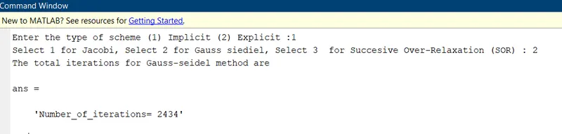
The iterations taken by each method are:
JACOBI
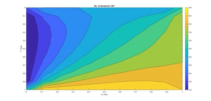

GAUSS SIEDEL
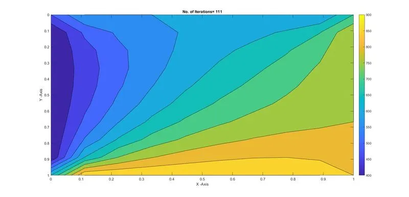

Successive Over- Relaxation (SOR)

II) Unsteady 2D heat conduction MATLAB code was written as follows
1. The temperature array is established when the inputs are defined as variables.
2. Boundary conditions are inserted into the temperature array, and boundary values are averaged at corners.
3. To conduct the iteration, constants such as alpha, omega, and tolerance are defined.
4. A user must supply one or two inputs here.
a) The first input is whether the problem should be solved explicitly or implicitly.
b) If an implicit approach is chosen, the user must give additional information in order to select the iterative strategy.
The if-else loop is used to solve the equation iteratively using the selected (user input) approach.
c) The for loop is used to repeat the iteration several times in order to achieve steady-state conditions.
d) The while loop is used to iteratively run the scheme selected until the requisite precision is attained.
At each iterative phase, two for loops are utilized to calculate the temperature values at each node.
clear all
close all
clc

% Unsteady 2D heat conduction

% defining domain and discretizing
length=1; % length of 1m
n_nodes = 10 ;% number of nodes
x= linspace(0,length,n_nodes);
y= linspace (0,length,n_nodes);
dx= length/n_nodes;
dy= length/n_nodes;
dt=1/10;

% defining initial temperature at all nodes at 300K
T=300*ones(n_nodes,n_nodes);
T(1:end,1)= 400 ; % left side boundary  at 400K
T(1:end,end)= 800 ; % right side boundary at 800K
T(end,1:end) = 900 ; % bottom boundary at 600K
T(1,1:end) = 600 ; % top boundary at 600K

% Average value of T at corners
T(1,1)=500 ;
T(1,end)= 700;
T(end,1)= 650 ;
T(end,end)= 850;

% Storing the value of T
T_old = T; % for previous space term
T_time= T ; % for previous time step

% Giving constant values
K = (2*(dx^2+dy^2))/(dx^2*dy^2);
omega= 1.15; %
a = 1.5 ; % alpha value
k1= (a*dt)/(dx^2);
k2 = (a*dt)/(dy^2);
iter = 0;

scheme = input('Enter the type of scheme (1) Implicit (2) Explicit :');

if scheme==1
    method = input('Select 1 for Jacobi, Select 2 for Gauss siediel, Select 3  for Succesive Over-Relaxation (SOR) : ');
if method == 1 % For jacobi method
    for t=1:2000
        error=10;
        tol = 1e-4;
    while(error>tol)
        for i = 2:n_nodes-1
            for j = 2:n_nodes-1
            term1 = 1/(1+(2*k1)+(2*k2));
            term2 = k1*(T_old(i+1,j) + T_old(i-1,j));
            term3 = k2*(T_old(i,j+1)+ T_old(i,j-1));
            T(i,j) = term1*(T_time(i,j)+term2+term3);
            end
        end
        iter = iter + 1;
        error=max(max((abs(T_old-T))));
        T_old=T;
    end
    T_time=T;
    end
    disp('The total iterations for Jacobi method are')
elseif method==2
    for t=1:2000
        error=10;
        tol = 1e-4;
    while(error>tol)
        for i = 2:n_nodes-1
            for j = 2:n_nodes-1
            term1 = 1/(1+(2*k1)+(2*k2));
            term2 = k1*(T_old(i+1,j)+ T(i-1,j));
            term3 = k2*(T_old(i,j+1)+ T(i,j-1));
            T(i,j) = term1*(T_time(i,j)+term2 + term3);
            end
        end
        iter=iter+1;
        error=max(max((abs(T_old-T))));
        T_old=T;
    end
    T_time=T;
    end
    disp('The total iterations for Gauss-seidel method are')
else
    for t=1:2000
        error=10;
        tol = 1e-4;
         while(error>tol)
            for i = 2:n_nodes-1
                for j = 2:n_nodes-1
            term1 = 1/(1+(2*k1)+(2*k2));
            term2 = k1*(T_old(i+1,j)+ T(i-1,j));
            term3 = k2*(T_old(i,j+1)+ T(i,j-1));
            term4 = term1*(T_time(i,j)+term2+term3);
            T(i,j) = (1-omega)*T_old(i,j)+(omega*term4);
                end
            end
        iter=iter+1;
        error=max(max((abs(T_old-T))));
        T_old=T;
    end
    T_time=T;
    end
    disp('The total iterations for SOR method are')
end
else
    for t=1:2000
        for i = 2:n_nodes-1
            for j = 2:n_nodes-1
            term1 = k1*(T_time(i+1,j)-2*T_time(i,j)+T_time(i-1,j));
            term2 = k2*(T_time(i,j+1)-2*T_time(i,j)+T_time(i,j-1));
            T(i,j) = T_time(i,j)+term2+term1;
            end
        end
        T_time=T;
        iter=iter+1;
    end
end
% displaying the reults

sprintf('Number_of_iterations= %d', iter)

% Plotting the reults

[X,Y]=meshgrid(x,y);
figure(1)
contourf(X,Y,T)
colorbar
set(gca,'ydir','reverse')

xlabel('X -Axis')
ylabel('Y -Axis')
title(sprintf('No. of Iterations= %d',iter));
pause(0.02)
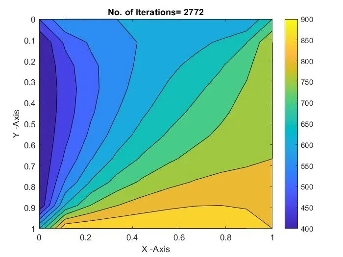
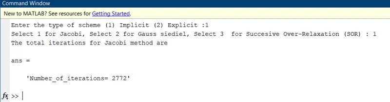
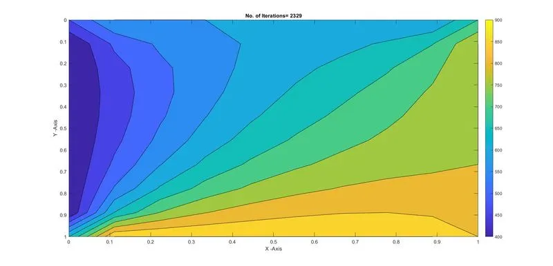
The results are as follows for all the methods:
1) Jacobi
2) Gauss Siedel
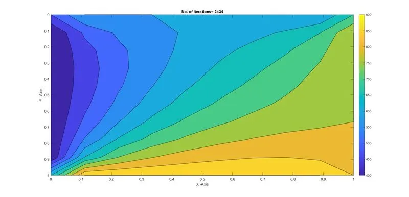
3) SOR
CONCLUSION:
The program was completed successfully. The temperature distribution map obtained is the same for both steady and unstable situations because the solution approaches steady-state in the transient analysis as well. The amount of iterations required to reach a solution is compared between the three iterative approaches. The Successive over-relaxation method requires fewer iterations in both steady and transient analysis. The number of iterations taken by Successive over RelaxationNumber of iterations is lowest followed by Gauss-SiedelNumber and it is highest for the Jacobi method.
Explicit and Implicit results differ in that the latter part does not rely heavily on the Courant number for stability and convergence, whereas in the Explicit approach, information from a given cell or mesh element must propagate to its immediate neighbors, so a low CFL number must be considered.