Week 5.1 - Mid term project - Solving the steady and unsteady 2D heat conduction problem
Objective: To solve the 2D heat conduction equation under steady and transient conditions using the explicit and implicit methods.
Explicit and Implicit Methods:
Explicit methods calculate the state of a system at a later time from the state of the system at the current time, while implicit methods find a solution by solving an equation involving both the current state of the system and the later one.
Heat Conduction Equation:
The heat conduction equation is a partial differential equation that describes the distribution of heat (or the temperature field) in a given body over time.
Part 1: Steady-state heat conduction:
Input conditions to solve 2D heat conduction at steady state using implicit techniques:
Length: 1m
Grid points along with x-axis i.e: 100
Grid points along with y-axis i.e: 100
Temperature at Left = 400k
Temperature at Right = 500k
Temperature at Top = 600k
Temperature at Bottom = 900k
`omega`= 1.25
2D Heat conduction steady-state equation and its solvers:
|
Implicit Iterative solver |
Steady State |
|
`(del^2T)/(delx^2)+(del^2T)/(dely^2)=0` |
|
|
`(del^2T)/(delx^2)=(T(i-1,j)+2T(i,j)+T(i+1,j))/(deltax^2)` `(del^2T)/(dely^2)=(T(i,j-1)+2T(i,j)+T(i,j+1))/(deltay^2)` Note: Heat conduction equation expanded using second order central differencing method |
|
|
1 |
Jacobi |
|
`T(i,j)=((T(i-1,j)+T(i+1,j))/(k*dx^2) +(T(i,j-1)+T(i,j-1))/(k*dy^2))^(old)` where `k=(2(delx^2+dely^2))/(delx^2*dely^2)` |
|
|
2 |
Gauss Seidel |
|
`T(i,j)=((T(i-1,j)^(old)+T(i+1,j))/(k*dx^2) +(T(i,j-1)^(old)+T(i,j-1))/(k*dy^2) )` where `k=(2(delx^2+dely^2))/(delx^2*dely^2)` |
|
|
3 |
Successive Over Relaxation |
|
`T(i,j)=(1-omega)T(i,j)^(old)+omega((T(i-1,j)^(old)+T(i+1,j))/(k*dx^2) +(T(i,j-1)^(old)+T(i,j-1))/(k*dy^2) )` where `k=(2(delx^2+dely^2))/(delx^2*dely^2)` |
Program to solve the 2D Heat Conduction at steady state using Implicit techniques:
clear all
close all
clc
L=1%Length of the domain
omega=1.25% SOR factor
nx=100%grid size
ny=nx
x=linspace(0,L,nx)
dx=x(2)-x(1)
y=linspace(0,L,ny)
dy=y(2)-y(1)
T=300*ones(nx,ny)
T(:,1)=400;
T(1,:)=900;
T(:,end)=800;
T(end,:)=600;
T(1,1)=(900+400)/2;
T(1,end)=(900+800)/2;
T(end,1)=(400+600)/2;
T(end,end)=(800+600)/2;
Told=T
k1=2*(dx^2+dy^2)/(dx^2*dy^2)
tol=1e-4;
error=9e9;
solver=input('Enter the number for the solver method: \n Jacobi=1 \n Gauss Seidel=2 \n SOR=3 \n Solver Type: ');
if solver == 1
   tic
   jacobi_iter=1;
   while (error>tol)
    for j=2:ny-1
      for i=2:nx-1
        H=((Told(i-1,j)+Told(i+1,j))/(k1*dx^2));
        V=((Told(i,j-1)+Told(i,j+1))/(k1*dy^2));
        T(i,j)=H+V;
      end
    end
    error=max(max(abs(Told-T)))
    Told=T;
    jacobi_iter=jacobi_iter+1
    timecounter=toc;
    figure(1)
    [C,h]=contourf(x,y,T,'ShowText','on');
    colorbar
    colormap(jet)
    xlabel('xx');
    ylabel('yy');
    clabel(C,h)
    title(sprintf('2d Steady State Heat Conduction  \n Method:Jacobi \n No of iterations=%d \n Time:%f s',jacobi_iter,timecounter))
   end
end
   if solver == 2
   tic
   gs_iter=1;
   while (error>tol)
    for j=2:ny-1
      for i=2:nx-1
        H=((T(i-1,j)+Told(i+1,j))/(k1*dx^2));
        V=((T(i,j-1)+Told(i,j+1))/(k1*dy^2));
        T(i,j)=H+V;
      end
    end
    error=max(max(abs(Told-T)))
    Told=T;
    gs_iter=gs_iter+1
    timecounter_1=toc;
    figure(1)
    [C,h]=contourf(x,y,T,'ShowText','on');
    colorbar
    colormap(jet)
    xlabel('xx');
    ylabel('yy');
    clabel(C,h)
    title(sprintf('2d Steady State Heat Conduction  \n Method:Gauss Seidel \n No of iterations=%d \n Time:%f s',gs_iter,timecounter_1))
   end
   end
      if solver == 3
   tic
   sor_iter=1;
   while (error>tol)
    for j=2:ny-1
      for i=2:nx-1
        H=((T(i-1,j)+Told(i+1,j))/(k1*dx^2));
        V=((T(i,j-1)+Told(i,j+1))/(k1*dy^2));
        T(i,j)=(Told(i,j)*(1-omega))+(omega*(H+V));
      end
    end
    error=max(max(abs(Told-T)))
    Told=T;
    sor_iter=sor_iter+1
    timecounter_2=toc;
    figure(1)
    [C,h]=contourf(x,y,T,'ShowText','on');
    colorbar
    colormap(jet)
    xlabel('xx');
    ylabel('yy');
    clabel(C,h)
    title(sprintf('2d Steady State Heat Conduction  \n Method:SOR \n No of iterations=%d \n Time:%f s',sor_iter,timecounter_2))
   end
   end
Result:
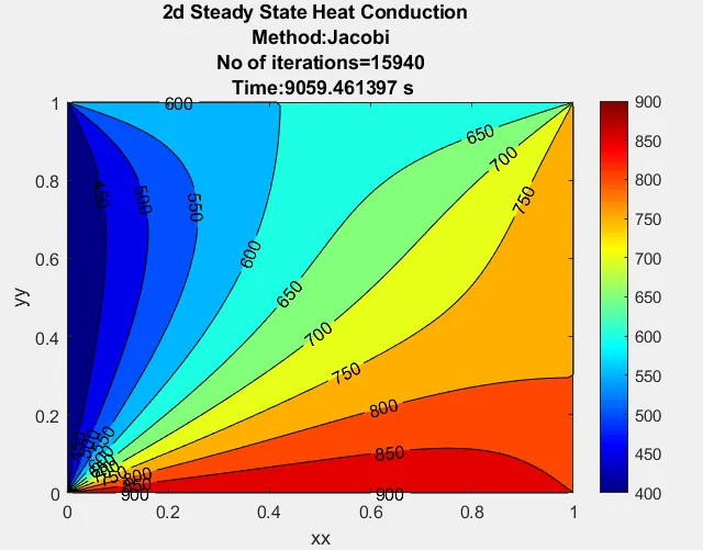
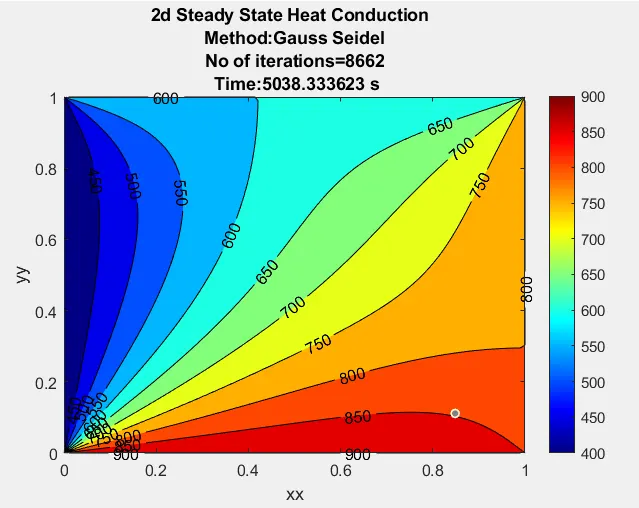
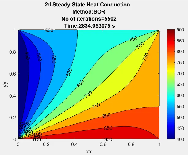
Part 2: Transient-state heat conduction
Input conditions to solve 2D heat conduction under transient state using implicit & explicit techniques:
Length: 1m
Grid points along with x-axis i.e: 51
Grid points along with y-axis i.e: 51
Temperature at Left = 400k
Temperature at Right = 500k
Temperature at Top = 600k
temperature at Bottom = 900k
`omega`= 1.3
`alpha`=1e-4
2D Heat conduction transient-state equation and its solvers:
|
Transient State |
||
|
`(del T)/(delt)=alpha((del ^2T)/(delx^2)+(del ^2T)/(dely^2))` |
||
|
`(del^2T)/(delx^2)=(T(i-1,j)+2T(i,j)+T(i+1,j))/(deltax^2)` `(del^2T)/(dely^2)=(T(i,j-1)+2T(i,j)+T(i,j+1))/(deltay^2)` Note: Heat conduction equation expanded using second order central differencing method |
||
|
1. Explicit |
||
|
1. `T(i,j)^(n)=(1-2kunderset(1)()-2kunderset(2)())*T(i,j)^(n-1)+kunderset(1)()*(T(i-1,j)+T(i.j-1))^(n-1)+kunderset(2)()*(T(i,j-1)+T(i.j+1))^(n-1)` Where `kunderset(1)()=(alpha*d^2t)/dx^2` `kunderset(2)()=(alpha*d^2t)/dy^2` |
||
|
2. Implicit - Jacobi |
||
|
`term 1 = 1/(1+2kunderset(1)()+2kunderset(2)())` `term 2 = k1*term 1` `term 3 = k2*term 1` `T(i,j)^n=term1*T(i,j)^(n-1)+term2*(T(i-1,j)+T(i+1,j))^(old)+term3*(T(i,j-1)+T(i,j+1))^(old)` |
||
|
3. Implicit – Gauss seidel |
||
|
`term 1 = 1/(1+2kunderset(1)()+2kunderset(2)())` `term 2 = k1*term 1` `term 3 = k2*term 1` `T(i,j)^n=term1*T(i,j)^(n-1)+term2*(T(i-1,j)+T(i+1,j)^(old))+term3*(T(i,j-1)+T(i,j+1)^(old))` |
||
|
Program to solve Transient state heat conduction equation: Explicit
%% 2D Transient State Heat Conduction Equation solved using explicit Method
clear all;
close all;
clc;
%% Initializing Variables:
Nx = 51;
Ny = 51;
x = linspace(0,1,Nx);
y = linspace(0,1,Ny);
dx = 1/(Nx-1);
dy = 1/(Ny-1);
alpha = 0.0001;
dt = 1;

tol = 1e-4;

%% Initializing the Temperature grid:
T = 298*ones(Nx,Ny);
T(1,:) = 900; % Bottom Temperature
T(end,:) = 600; % Top Temperature
T(:,1) = 400; % Left Temperature
T(:,end) = 800; % Right Temperature
% Edge refining
T(1,1) = (900+400)/2;
T(1,end) = (900+800)/2;
T(end,1) = (400+600)/2;
T(end,end) = (800+600)/2;

%% CFL Number calculation and adaptive Time-step control:
CFL_Number = (alpha*dt)*((1/dx^2)+(1/dy^2));

%% Calculation of Temperature Distribution explicitly using iterative solvers:

k1 = (alpha*dt)/(dx^2);
k2 = (alpha*dt)/(dy^2);
[xx,yy] = meshgrid(x,y);
Told = T;
T_prev_dt = T;
tic;
counter = 1;
for z = 1:2500
    %% explicit Iteration Scheme
    for i = 2:Nx-1
        for j = 2:Ny-1
            term1 = (1-2*k1-2*k2)*Told(i,j);
            term2 = k1*(Told(i-1,j)+Told(i+1,j));
            term3 = k2*(Told(i,j-1)+Told(i,j+1));
            T(i,j) = term1+term2+term3;
        end
    end
    Told = T;
    counter = counter+1;
    time_counter = toc;
figure(1)
[C,h] = contourf(xx,yy,T);
colorbar;
colormap(jet);
clabel(C,h);
title(sprintf('2D Unsteady state heat conduction \n Method:Explicit Method \n Number of iterations: %d (Time: %0.2fs) \n Computation Time: %0.4f \n CFL Number: %0.4f',counter-1,z*dt,time_counter,CFL_Number));
xlabel('xx');
ylabel('yy');
end
Result:
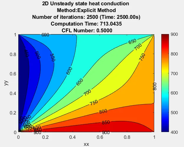
%% 2D Transient State Heat Conduction Equation solved using Implicit Method
clear all;
close all;
clc;
%% Initializing Variables:
Nx = 51;
Ny = 51;
x = linspace(0,1,Nx);
y = linspace(0,1,Ny);
dx = 1/(Nx-1);
dy = 1/(Ny-1);
alpha = 0.0001;
dt =1;
tol = 1e-4;
%% Initializing the Temperature grid:
T = 298*ones(Nx,Ny);
T(1,:) = 900; % Bottom Temperature
T(end,:) = 600; % Top Temperature
T(:,1) = 400; % Left Temperature
T(:,end) = 800; % Right Temperature
% Edge refining
T(1,1) = (900+400)/2;
T(1,end) = (900+800)/2;
T(end,1) = (400+600)/2;
T(end,end) = (800+600)/2;
%% CFL Number calculation:
CFL_Number = alpha*dt*((1/dx^2)+(1/dy^2));

%% Calculation of Temperature Distribution Implicitly using iterative solvers:

k1 = (alpha*dt)/(dx^2);
k2 = (alpha*dt)/(dy^2);
[xx,yy] = meshgrid(x,y);
Told = T;
T_prev_dt = T;
   term1 = 1/(1+2*k1+2*k2);
   term2 = k1*term1;
   term3 = k2*term1;
tic;
counter = 1;
solver=input('Enter the number for the solver method: \n Jacobi=1 \n Gauss Seidel=2 \n SOR=3 \n Solver Type: ');
if solver == 1
for k=1:2500
    error = 9e9;
    while(tol<error)
     for j = 2:Ny-1
        for i = 2:Nx-1
            H= (Told(i-1,j)+Told(i+1,j));
            V= (Told(i,j-1)+Told(i,j+1));
            T(i,j) =(T_prev_dt(i,j)*term1)+(H*term2)+(V*term3);
        end
      end
     error=max(max(abs(Told-T)))
     Told = T;
     counter = counter+1;
     end
     T_prev_dt = T
     figure(1)
     [C,h] = contourf(xx,yy,T);
     colorbar;
     colormap(jet);
     clabel(C,h);
     time_counter = toc;
     title(sprintf('2D Unsteady state heat conduction \n Method:Implicit Jacobi \n Number of iterations: %d (Time: %0.2fs) \n Computation Time: %0.4f \n CFL Number: %0.4f',counter-1,k*dt,time_counter,CFL_Number));
     xlabel('xx');
     ylabel('yy');
end
end

if solver == 2
for k=1:2500
    error = 9e9;
    while(tol<error)
     for j = 2:Ny-1
        for i = 2:Nx-1
            H= (T(i-1,j)+Told(i+1,j));
            V= (T(i,j-1)+Told(i,j+1));
            T(i,j) =(T_prev_dt(i,j)*term1)+(H*term2)+(V*term3);
        end
      end
     error=max(max(abs(Told-T)))
     Told = T;
     counter = counter+1;
     end
     T_prev_dt = T
     figure(1)
     [C,h] = contourf(xx,yy,T);
     colorbar;
     colormap(jet);
     clabel(C,h);
     time_counter = toc;
     title(sprintf('2D Unsteady state heat conduction \n Method:Implicit Gauss Seidel \n Number of iterations: %d (Time: %0.2fs) \n Computation Time: %0.4f \n CFL Number: %0.4f',counter-1,k*dt,time_counter,CFL_Number));
     xlabel('xx');
     ylabel('yy');
end
end

if solver == 3
for k=1:2500
    error = 9e9;
    while(tol<error)
     for j = 2:Ny-1
        for i = 2:Nx-1
            H= (T(i-1,j)+Told(i+1,j));
            V= (T(i,j-1)+Told(i,j+1));
            T(i,j) =(1-1.3)*(Told(i,j))+(1.3*((T_prev_dt(i,j)*term1)+(H*term2)+(V*term3)));
        end
      end
     error=max(max(abs(Told-T)))
     Told = T;
     counter = counter+1;
     end
     T_prev_dt = T
     figure(1)
     [C,h] = contourf(xx,yy,T);
     colorbar;
     colormap(jet);
     clabel(C,h);
     time_counter = toc;
     title(sprintf('2D Unsteady state heat conduction \n Method:Implicit SOR \n Number of iterations: %d (Time: %0.2fs) \n Computation Time: %0.4f \n CFL Number: %0.4f',counter-1,k*dt,time_counter,CFL_Number));
     xlabel('xx');
     ylabel('yy');
end
end
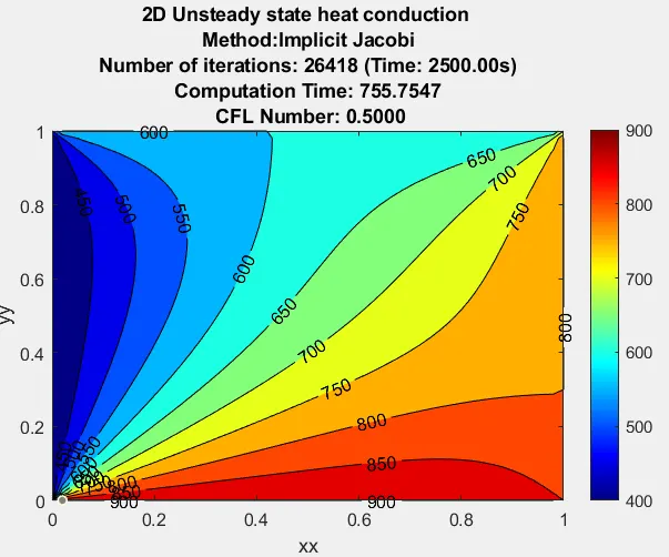
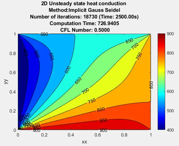
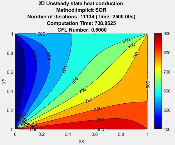
Result:
Conclusion:
Part 1: Steady-state heat conduction
From the above results, the iteration for convergence of plot is very high for the Jacobi method when compared with Gauss-Seidel & SOR. By increasing the grid size we can drastically reduce the iterations which as well gives a convergence plot with stability.
Part 2: Transient-state heat conduction
The above results show the convergence of transient heat equation using explicit and implicit techniques
1. Unsteady state problems can be solved by both implicit and explicit methods.
2. For stiff equations requires lesser timesteps and larger computation time to solve using explicit method.
3. Among implicit solvers SOR gives the result in less time compared to other techniques. It gives a stable result irrespective of the CFL number.