Week 5.1 - Mid term project - Solving the steady and unsteady 2D heat conduction problem
AIM:
- To solve the 2D heat conduction problem for the steady and unsteady state using Jacobi, gauss seidel, and successive over-relaxation iterative techniques.
THEORY:
- Conduction is a mode of heat transfer, generally takes place in solids due to temperature differences associated with free electron and lattice vibration.
- A generalized conduction equation is given
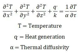
- Thermal diffusivity is a thermophysical property of a material defined as the ratio of thermal conductivity of the material and its thermal capacity.
- Since the problem is 2D and there is no heat generation is considered, therefore those terms are neglected. So the equation represents the unsteady 2D heat conduction (parabolic).
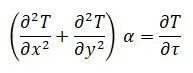
For steady-state, time derivative is not considered, their fore below equation represents the 2D steady-state Heat conduction (elliptic).
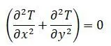
- Difference equations for the steady-state and unsteady-state 2D conduction equation are derived to obtain the numerical solution.
| Steady State 2D heat conduction | 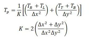 |
| Transient 2D heat conduction (explicit) | 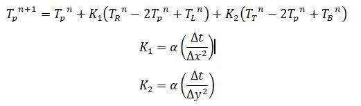 |
| Transient 2D heat conduction (implicit) | 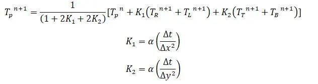 |
- Here iterative methods are used to solve the difference equation, Iterative methods are numerical techniques used to converge the solution(accurately) of a problem with some initial guess.
- Here Jacobi, gauss-seidel, and successive over-relaxation techniques are used.
MATLAB CODE:
- There is 2 Matlab code written separately for steady and unsteady conditions.
- But for both conditions inputs are the same
- while programming it is assumed that, the domain is the surface of area (1mX1m). Discretized into 10 nodes both horizontally and vertically.
- Constant values like alpha and time step 'data, by keeping the explicit condition in mind.
- relaxation factor omega is also assumed while programming only.
Inputs
| Top boundary temperature | 600 K |
| Bottom Boundary temperature | 900 K |
| Left Boundary temperature | 400 K |
| Right Boundary temperature | 800 K |
| error | 1e-4 |
Steady-State 2D Heat conduction
- First inputs are defined into variables and the temperature array is created.
- Boundary conditions are introduced into the temperature array, and at corners, boundary values are averaged.
- Constants like alpha, omega, tolerance are defined to run the iteration.
- Input must be provided by the user, to choose the iterative method.
- The if-else loop is used to solve the equation using the selected(input from the user) iterative technique.
- while loop is used to run the iterative technique till the required accuracy is achieved.
- Two for loop is used to calculate the temperature values at every node at each iterative step.
close all
clear all
clc


            % Domain and discretization length

             Number _node  =  10;

             domain_length = 1;

             %value of x and y at nodes in a discretization   plan

             x =  linspace(0,domain_length,number_node);

             y = linspace(0,domain_length,number_node);

             dx = domain_length (number _ node -1);

             dy = domain_length( number_ node-1);

             % Let define a temperature value at all nodes with initial guess 300k

             T = 300 * ones(number _ node, number_ node);

             % Initial boundary conditions at left and right

             T(1:end,1) = 400;

             T(1:end,end) = 800;

             % Initial boundary conditions at bottom and top

             T(end,1:end)  = 900;
             T(1,1: end) = 600;


              % average values of T at corner boundaries:


                    T(1, 1 )  = 500;

                     T(end, 1 )  = 650;

                    T(1, end )  = 700;

                    T(end, end )  = 850;


               %copy of Temperature to compute to compute

         T_ old = T;


         %constant

         K = (2*(dx^2 + dy^2))/(dx^2*dy^2);

         omegha = 1.2;

         % to enter while loop initialize error value randomly

         error = 10;

         tol = 1e-4;

         no _ iteration = 0;

         method = input(‘enter(1) for jacobi,(2) for gauss siediel,(3) for sos’);

         if method == 1

           while(error>>tol)

                for i = 2:number_node-1

                   for j . 2:numher_node-1

                   term 1 = (T _old(i+1,j )+T _ old(i-1,j))/ dx^2;

                   term 2 = (T _old(i,j+1 )+T _ old(i,j-1))/ dy^2;

                       T(i,j) =  (term1 + term 2)/K;

                   end


                end

                error = max(max(abs(T_ old _ T)));

                 % to update the previous velocity with new velocity

                 %got from the iteration

                 T_ old = T;

                 no_iteration = no_iteration+1;

             end

          elseif method

             while(error>to1)

                 for i = 2:number_node-1

                 for j  = 2: number _ node-1

    term 1 = (T _old(i+1,j )+T _ old(i-1,j))/ dx^2;

   term 2 = (T _old(i,j+1 )+T _ old(i,j-1))/ dy^2;

        T(i,j) =  (term1 + term 2)/K;

               end

                   error = max(max(abs(T_ old _ T)));


                     % to update the previous velocity with new velocity

                          % got from the iteration

                 T_ old = T;

                 no_iteration = no_iteration+1;

             end

          elseif method

             while(error>to1)

                 for i = 2:number_node-1

                 for j  = 2: number _ node-1

    term 1 = (T _old(i+1,j )+T _ old(i-1,j))/ dx^2;

   term 2 = (T _old(i,j+1 )+T _ old(i,j-1))/ dy^2;

        T(i,j) =  (1-omega)*T_ old(i,j))  + omega (term 1 + term 2 ) / k);

               end

                   error = max(max(abs(T_ old _ T)));

                         % to update the previous velocity with new velocity

                          % got from the iteration

                             T_ old = T;

                              no_iteration = no_iteration+1;

                            end

                      end

                        % to visualize of result

                  [X, Y] = meshgrid(x,y);

                   Contour f(X,Y,T)

                    Color bar

                    Set (gca, ‘ ydir’, ‘reverse’,)
Unsteady-State 2D Heat conduction :-
- Inputs are defined into variables and the temperature array is created.
- Boundary conditions are introduced into the temperature array, and at corners, boundary values are averaged.
- Constants like alpha, omega, tolerance are defined to run the iteration.
- Here a user must provide, one or two inputs.
- The first input is to whether solve the problem using an explicit approach or an implicit approach.
- If an implicit approach is selected, then the user must provide another input, to select the iterative technique.
- The if-else loop is used to solve the equation using the selected(input from the user) approach and iterative technique.
 close all
             clear all
             clc

            % Domain and discretization length

            Number _node = 10;

             domain_length = 1;

             %value of x and y at nodes in a discretization   plane


             x =  linspace(0,domain_length,number_node);

             y = linspace(0,domain_length,number_node);


             dx = domain_length (number _ node -1);


             dy = domain_length( number_ node-1);


             % Let define a temperature value at all nodes with initial guess 300k


             T = 300 * ones(number _ node, number_ node);


             % Initial boundary conditions at left and right

             T(1:end,1) = 400;

             T(1:end,end) = 800;


             % Initial boundary conditions at bottom and top

             T(end,1:end)  = 900;

             T(1,1: end) = 600;


                 % average values of T at corner boundaries:


                    T(1, 1 )  = 500;

                     T(end, 1 )  = 650;

                    T(1, end )  = 700;

                    T(end, end )  = 850;


               %copy of Temperature to compute to compute

         T_ old = T;


                   % copy of T for previous time _ step

         %constant

          Alpha = 1.5 ;

         omega = 1.15;

            K 1 =  (alpha *  dt ) / dx^2;

            K2 = (alpha *dt ) / dy^2;

Iteration = 0;

         Approach = input( ‘Enter 1 for implicit or Enter 2 for explicit’)

         if approach  == 1

         if method == 1

for nt = 1: 1500

   error = 10;

      to1 = 1e-4;

           while(error>>to1)

                for i = 2:number_node-1

                   for j = 2:numher_node-1

                term 1 = 1 / 1+(2*k1) + (2*k2);

                   term 2 = k1* (T _ old(i+1, j) +T _ old(i-1,j));

                   term 3 = k2* (T _old (i, j+1 )+T _ old(i,j-1));

                       T(i,j) =  term 1 *(T _ prev (i,j) + term 2 + term 3);

                   end


                end

                iteration = iteration + 1;

                error = max(max(abs(T_ old _ T))));

                  T _ old = T;

                  End

                T _ Prev = T;


         End

           elseif method  == 2;

            for nt = 1:1500

             error = 10;

            to1  = 1 e-4;

             while (error>to1);

                               for i = 2:number_node-1

                 for j  = 2: number _ node-1

                    term 1 = 1 / 1+(2*k1) + (2*k2);

                   term 2 = k1* (T _ old(i+1, j) +T _ old(i-1,j));

                   term 3 = k2* (T _old (i, j+1 )+T _ old(i,j-1));

                       T(i,j) =  term 1 *(T _ prev (i,j) + term 2 + term 3);

                   end


                end

                iteration = iteration + 1;

                error = max(max(abs(T_ old _ T))));


                 T _ old = T;

                  end

                T _ Prev = T;


         End

           elseif method  == 2;

            for nt = 1:1500

             error = 10;

            to1  = 1 e-4;

             while (error>to1);


            for i = 2:number_node-1

                 for j  = 2: number _ node-1

                    term 1 = 1 / 1+(2*k1) + (2*k2);

                   term 2 = k1* (T _ old(i+1, j) +T _ old(i-1,j));

                   term 3 = k2* (T _old (i, j+1 )+T _ old(i,j-1));

                  term 4 =    term 1 *(T _ prev (i,j) + term 2 + term 3);

                       T(i,j) =  ( 1 – omega) *(T _ old (i,j) + (omega *  term 4);

                   end


                end

                iteration = iteration + 1;

                error = max(max(abs(T_ old _ T))));


           T _ old = T;

                  end

                T _ Prev = T;


end

end

else


            for nt = 1:1500

                       for i = 2:number_node-1

                         for j = 2:number_node-1

                 term 1 = k1* (T _ prev(i+1, j)  - 2*T _ prev(i,j) + T _ Prev (i – 1 , j)));

                   term 2 = k2* (T _ prev(i,j+1)  - 2*T _ prev(i,j) + T _ prev(i , j-1)));

                   T(i,j) =    (T _ prev (i,j) + term 1 + term 2);

end


end


                             % to update the previous time step value  with new time step value

                          % got from the iteration

                             T_ prev = T;

                              iteration = iteration+1;

                            end

                      end

                        % to visualize of result

                  [X, Y] = meshgrid(x,y);

                   Contour f(X,Y,T)

                    Color bar

                    Set (gca, ‘ ydir’, ‘reverse’,)
RESULT:-
- The program ran successfully.
- The temperature distribution plot obtained for both the steady and unsteady conditions is the same.
- Because in Transient analysis also, the solution approaches to steady-state.
- The number of iterations taken to converge to the solution is compared among the 3 iterative techniques.
- In both steady and transient analysis, the number of iteration by the Successive over-relaxation method is less