Week 5.1 - Mid term project - Solving the steady and unsteady 2D heat conduction problem

AIM:

1. Steady state analysis & Transient State Analysis

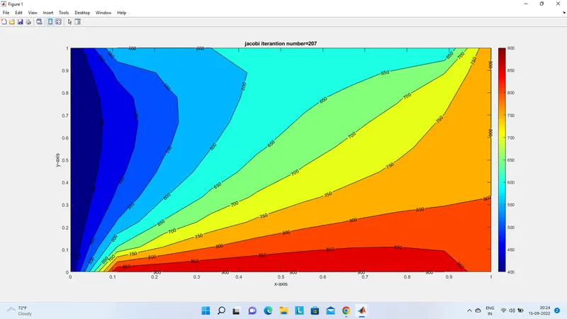
Solve the 2D heat conduction equation by using the point iterative techniques that were taught in the class. The Boundary conditions for the problem are as follows;

Top Boundary = 600 K

Bottom Boundary = 900 K

Left Boundary = 400 K

Right Boundary = 800 K

You will implement the following methods for solving implicit equations.

1. Jacobi

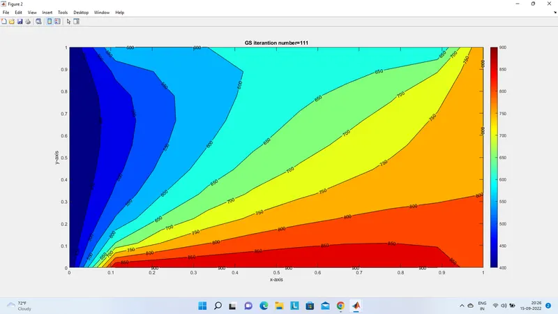
2. Gauss-seidel

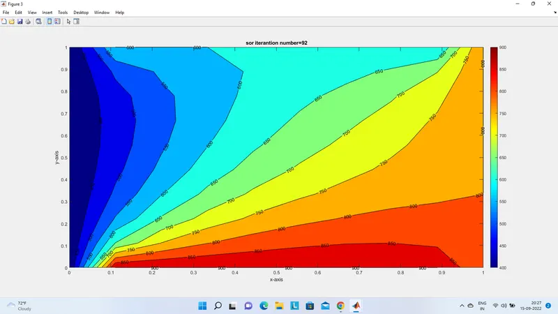
3. Successive over-relaxation

Your absolute error criteria is 1e-4

Make sure to use "INSERT CODE SAMPLE" option to paste the code here. Post screenshots of the plots and use the projects.skill-lync.com page to Publish your findings.

2. You will write code for both implicit and explicit schemes (This is for the Transient Analysis only)

3. Write a detailed explanation for your results, plots or codes without explanation 


Unsteady-State 2D Heat conduction

Inputs are defined into variables and the temperature array is created.
Boundary conditions are introduced into the temperature array, and at corners, boundary values are averaged.
Constants like alpha, omega, tolerance are defined to run the iteration.
Here a user must provide, one or two inputs.
The first input is to whether solve the problem using an explicit approach or an implicit approach.
If an implicit approach is selected, then the user must provide another input, to select the iterative technique.
The if-else loop is used to solve the equation using the selected(input from the user) approach and iterative technique.
For loop is used to run the iteration for a large number of times to reach steady-state conditions.
while loop is used to run the iterative technique till the required accuracy is achieved.
Two for loop is used to calculate the temperature values at every node at each iterative step.
Finally, a temperature distribution graph is obtained using 'conturf' command.

function code:


will awarded zero marks.function out = jacobi(t,told,i,j)
   out = 0.25*((told(i,j-1)+told(i,j+1)+told(i-1,j)+told(i+1,j)))
 end

function out = GS(t,told,i,j)
   out = 0.25*((t(i,j-1)+told(i,j+1)+t(i-1,j)+told(i+1,j)))
end



function out = sor(t,told,i,j,f)
  out = (1-f)*told(i,j) + f*(0.25*(t(i,j-1)+told(i,j+1)+t(i-1,j)+told(i+1,j)))
end
Main code

 Jacobi

clear all
close all
clc

% inputs
% number of grid points along x and y axis
nx= 10;
ny=10;
x=linspace(0,1,nx);
dx = x(2)-x(1);
y= linspace(0,1,ny);
z=fliplr(y);
f=1.1;
iter = 1;

t= 300*ones([nx,ny]);

% applying BC

t(1,:)=600;
t(end,:)=900;
t(:,1)=400;
t(:,end)=800;

% creating a copy
told=t;
r1=t;

error= 19;
tol = 1e-4;
for iterative_solver = 1:3;
    while(error>tol);
        for i=2:nx-1;
            for j=2:ny-1;
                if(iterative_solver==1);
                    t(i,j)= jacobi(t,told,i,j);
                elseif(iterative_solver==2)
                    t(i,j)=GS(t,told,i,j);
                elseif(iterative_solver==3)
                    t(i,j)= sor(t,told,i,j,f);
                end
            end
        end
        error = max(max(t-told));
        told = t;
        [u1,v1]=meshgrid(x,z);
        % plot
        
        if(iterative_solver==1);
            figure(1);
            contourf(u1,v1,t);
            [C,h]= contourf(u1,v1,t);
            colorbar;
            colormap(jet);
            clabel(C,h);
            xlabel('x-axis');
            ylabel('y-axis');
            title_text=sprintf('jacobi iterantion number=%d',iter);
            title(title_text);
            pause(0.003);
        elseif(iterative_solver==2);
            
            figure(2);
            contourf(u1,v1,t);
            [C,h]= contourf(u1,v1,t);
            colorbar;
            colormap(jet);
            clabel(C,h);
            xlabel('x-axis');
            ylabel('y-axis');
            title_text=sprintf('GS iterantion number=%d',iter);
            title(title_text);
            pause(0.003);
        else
            
            figure(3);
            [C,h]= contourf(u1,v1,t);
            colorbar;
            colormap(jet);
            clabel(C,h);
            xlabel('x-axis');
            ylabel('y-axis');
            title_text=sprintf('sor iterantion number=%d',iter);
            title(title_text);
            pause(0.003);
        end
        iter=iter+1;
    end
    error=19;
    iter=1;
    t=r1;
    told=t;
end
 Gauss-seidel

clear all
close all
clc

% inputs
% number of grid points along x and y axis
nx= 10;
ny=10;
x=linspace(0,1,nx);
dx = x(2)-x(1);
y= linspace(0,1,ny);
dy = y(2)-y(1);
f= 1.2;

t= ones(nx,ny)*298;
% applying BC

t(1,:)=600;
t(end,:)=900;
t(:,1)=400;
t(:,end)=800;

alpha= 1.4;
dt=0.001;

% defining k1 and k2
k1=alpha*(dt/dx^2);
k2=alpha*(dt/dy^2);

told=t;
t_initial=t;

for iterartive_solver = 1:3
    nt=1:1400;
    error=9e9;
    tol=1;
    tic;
    
    % iterartive_solver==1:3;
    iter=1;
    while error>tol
        for i=2:nx-1
            for j=2:ny-1
                term1= 1/(1+2*k1+2*k2);
                term2= k1*term1;
                term3= k2*term1;
                if iterartive_solver==1;
                    t(i,j)= ((told(i,j)*term1)+(term2*(t(i-1,j)+t(i+1,j))+(term3*(t(i,j-1)+t(i,j+1)))));
                elseif iterartive_solver==2;
                    t(i,j)= ((told(i,j)*term1)+(term2*(t(i-1,j)+told(i+1,j))+(term3*(t(i,j-1)+told(i,j+1)))));
                elseif iterartive_solver==3;
                    t(i,j)= (1-f)*told(i,j)+ f*(((told(i,j)*term1)+(term2*(t(i-1,j)+told(i+1,j))+(term3*(t(i,j-1)+told(i,j+1))))));
                end
            end
            error_n=max(abs(told-t));
            error=max(error_n);
            told=t;
            iter=iter+1;
            
        end
    end
    time=toc;
    
    %plot
    
    if iterartive_solver==1;
        figure(1)
        contourf(x,fliplr(y),t);
        [C,h]=contourf(x,fliplr(y),t);
        colorbar;
        colormap(jet);
        clabel(C,h);
        text = sprintf('JACOBI Method n iteration number = %d; t computational time: %0.4f',iter ,time);
        title(text);
        told=t_initial;
        t=t_initial;
    elseif iterartive_solver==2;
        
        figure(2)
        [c,h]=contourf(x,fliplr(y),t);
        colorbar;
        colormap(jet);
        clabel(c,h);
        title(sprintf('GS Method n iteration number = %d; t computational time: %0.4f',iter,time));
        told=t_initial;
        t=t_initial;
    else
        
        figure(3)
        [c,h]=contourf(x,fliplr(y),t);
        colorbar;
        colormap(jet);
        clabel(c,h);
        title(sprintf('SOR Method n iteration number = %d; t computational time: %0.4f',iter,time));
        told=t_initial;
        t=t_initial;
    end
end

 Successive over-relaxation

clear all
close all
clc

% inputs
% number of grid points along x and y axis
nx= 10;
ny=10;
x=linspace(0,1,nx);
dx = x(2)-x(1);
y= linspace(0,1,ny);
dy = y(2)-y(1);

c= 1;
% number of steps
nt=200;
% time steps
dt = 0.001;
% CFL number
k= (c*dt)/dx^2;

t= ones([nx,ny])*673;
% applying BC

t(1,:)=600;
t(end,:)=900;
t(:,1)=400;
t(:,end)=800;

told = t;

tic
iter=1
for p=1:nt
    for i= 2:nx-1
        for j=2:ny-1
            t(i,j)= k*(told(i-1,j)+told(i+1,j)+told(i,j+1)+told(i,j-1))+ (1-4*k)*told(i,j);
        end
    end
    error=max(abs(told-t));
    told=t;
    iter=iter+1;
end
    time = toc;
    figure(1)
    [c,h]=contourf(x,fliplr(y),t);
    colorbar;
    colormap(jet);
    clabel(c,h);
    title(sprintf('2D unsteady heat conduction (Explicit method) n iteration number=%d; t computational time :%0.4f',iter,time));
    xlabel('xx');
    ylabel('yy');

Result:

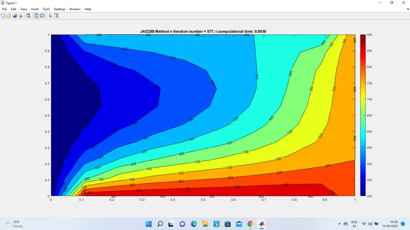
for jacobi method:

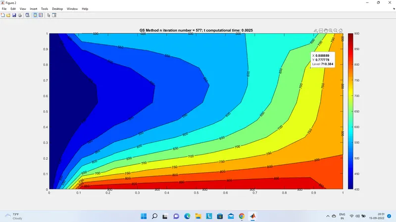
for GS method:

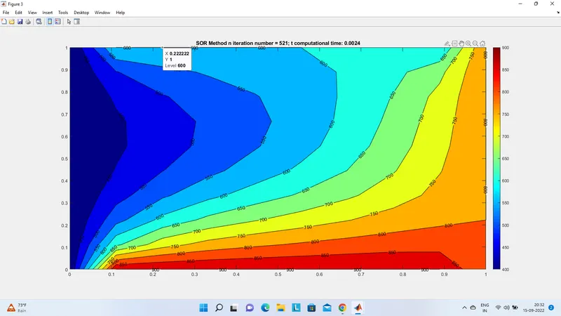
for SOR method:

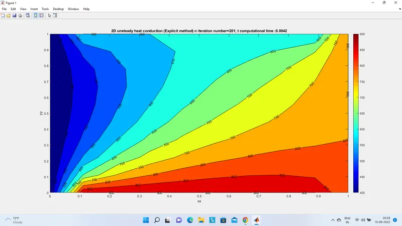
2D Unstady heat conduction

Plots:

for Jacobi:

for GS:

for SOR:

Explanation:

While comparing both Explicit and Implicit methods results, the Explicit method is much quicker than the implicit method.

The Explicit method takes 201 iterations whereas the Implicit method takes 577, 577, 521 iterations.

Coming to the implicit method SOR is the fastest method while comparing it with Jacobi and GS. The SOR method took 521 iterations.

But the Implicit method is more accurate as it uses various iterative solvers.