Week 5.1 - Mid term project - Solving the steady and unsteady 2D heat conduction problem
AIM:
To solve the steady and unsteady state 2D heat conduction equation using point iterative techniques.
ASSUMPTIONS:
Boundary Conditions:
Top Boundary = 600 K
Bottom Boundary = 900 K
Left Boundary = 400 K
Right Boundary = 800 K
Length of the Domain = 1 m
Thermal Diffusivity = 0.3 `m^2/s`
Tolerance criteria : 1e-4
THEORY:
The 2D unsteady heat conduction equation is :
```(del^2T)/(delx^2)+(del^2T)/(dely^2)= 1/alpha*(delT)/(delt)` ..................(1)
Since the above equation is elliptic in nature, we can discretize the space terms using central differencing scheme. But the time derivative can be discretized using either time IMPLICIT or EXPLICIT scheme. Time implicit scheme can be solved using iterative solvers like Jacobi, Guass-siedel and Successive Over Relaxation (SOR).
`(del^2T)/(delx^2)+(del^2T)/(dely^2)= 1/alpha*(delT)/(delt)`
`(T_(i+1,j)^(n) -2 T_(i,j)^n+T_(i-1,j)^n)/(Deltax)^2 + (T_(i,j+1)^(n) -2 T_(i,j)^n+T_(i,j-1)^n)/(Deltay)^2= 1/alpha* ((T_(i,j)^(n+1) -T_(i,j)^n)/(Deltat))` .........................................................(2)
Let,`k1= (alpha*Deltat)/(Deltax)^2 and k2=(alpha*Deltat)/(Deltay)^2`
On further simplication of eqn.(1)
`T_(i,j)^(n+1) = (T_(i,j)^n+k1*(T_(i+1,j)+T_(i-1,j))^n+k2*(T_(i,j+1)+T_(i,j-1))^n)/(1+2k1+2k2)`
On futher subsitution into the iterative solvers i.e., Jacobi, Gauss-Siedel and SOR, our implicit equation takes the form as follows:
Jacobi:
`T_(i,j)^(n+1) = (T_(i,j)^n+k1*(T_(i+1,j)+T_(i-1,j))^n+k2*(T_(i,j+1)+T_(i,j-1))^n)/(1+2k1+2k2)`
Gauss-Siedel:
`T_(i,j)^(n+1) = (T_(i,j)^(n+1)+k1*(T_(i+1,j)+T_(i-1,j))^(n+1)+k2*(T_(i,j+1)+T_(i,j-1))^(n+1))/(1+2k1+2k2)`
SOR:
`T_(i,j)^(n+1) = (1-omega)*T_(i,j)^n + omega*((T_(i,j)^n+k1*(T_(i+1,j)+T_(i-1,j))^(n+1)+k2*(T_(i,j+1)+T_(i,j-1))^(n+1))/(1+2k1+2k2)`
where `omega` is the relaxation factor.
Now for explicit scheme, we calculate the state of a system a later time from the current state of the system at the current time.
`T_(i,j)^(n+1) = T_(i,j)^n+k1*(T_(i+1,j)-2T_(i,j)+T_(i-1,j))^n+k2*(T_(i,j+1)-2T_(i,j)+T_(i,j-1))^n`
Similarily for the steady state heat cconduction equation, the same iterative solver can be employed to solve for the temperature.Eqn.(3) give the governing differential equation for 2D steady state heat conduction equation.
`(del^2T)/(delx^2)+(del^2T)/(dely^2)= 0`...........................(3)
Eqn.(3) can be disccretized using central differencing scheme due to its elliptic nature of the PDE.
The discretized equation is as follows:
`(T_(i+1,j)-2T_(i,j)+T_(i-1,j))^n/(Deltax)^2 + (T_(i,j+1)-2T_(i,j)+T_(i,j-1))^n/(Deltay)^2=0`
`T_(i,j)*(2 ((Deltax)^2+(Deltay)^2))/((Deltax)^2*(Deltay)^2)= (T_(i+1,j)+T_(i-1,j))/(Deltax)^2 + (T_(i,j+1)+T_(i,j-1))/(Deltay)^2`
Let, `k =(2 ((Deltax)^2+(Deltay)^2))/((Deltax)^2*(Deltay)^2)`
`implies``T_(i,j) = (1/k)*(T_(i+1,j)+T_(i-1,j))/(Deltax)^2 + (T_(i,j+1)+T_(i,j-1))/(Deltay)^2`
Now incorporating this discretized equation to iterative solver implies:
Jacobi:
`T_(i,j)^(n+1) = (1/k)*(T_(i+1,j)+T_(i-1,j))^n/(Deltax)^2 + (T_(i,j+1)+T_(i,j-1))^n/(Deltay)^2`
Gauss-Siedel:
`T_(i,j)^(n+1) = (1/k)*(T_(i+1,j)+T_(i-1,j))^(n+1)/(Deltax)^2 + (T_(i,j+1)+T_(i,j-1))^(n+1)/(Deltay)^2`
SOR:
`T_(i,j)^(n+1) = T_(i,j)^n*(1-omega) + omega*(1/k*(T_(i+1,j)+T_(i-1,j))^(n+1)/(Deltax)^2 + (T_(i,j+1)+T_(i,j-1))^(n+1)/(Deltay)^2)`
where, `omega` is the relaxation factor.
SOLUTION:
The above equation are coded in Octave and solved.
Code for Steady State 2D Heat Conduction equation:
% Steady state 2D Heat Conduction equation
% Iterative solvers- Jacobi,Gauss-siedel,Successive Over relaxation(SOR)
nx = ny = 20;
x = linspace(0,1,nx);
y = linspace(0,1,ny);
dx = x(2)-x(1);
dy = y(2)-y(1);

%Initial Temeperature Conditions

T = 300*ones(nx,ny);
T(1,:) = 600;
T(:,1) = 400;
T(nx,:) = 900;
T(:,ny) = 800;
T(1,1) = 500;
T(nx,ny)=850;
T(nx,1) = 650;
T(1,ny) = 700;
Told = T;
dt = 1e-3; %Time step size
tol = 1e-4;
nt = 1500; % No. of time steps
k = (2*((dx^2)+(dy^2))/((dx^2)*(dy^2)));
w  = 1.5; %Relaxation Factor
method = input('Iterative method = ') %iterative solver selection
if (method==1) %%Jacobi
  jacobi_iter = 1;
  error = 100;
    while(error>tol)
      for i=2:(nx-1)
        for j=2:(ny-1)
          H = (Told(i-1,j)+Told(i+1,j))/(dx^2);
          V = (Told(i,j-1)+Told(i,j+1))/(dy^2);
          T(i,j)= (1/k)*(H+V);
        endfor
      endfor
  error=max(max(abs(Told-T)));
  Told = T;
  jacobi_iter = jacobi_iter+1;
   end
% Plotting the graph
figure(1)
colormap(jet);
A=contourf(x,y,T);
clabel(A);
colorbar;
set(gca,'YDir','reverse');
xlabel('X');
ylabel('Y');
text1 = sprintf('Number of iterations = %d',jacobi_iter);
title({'Steady State Heat Conduction Solver - Jacobi';text1});
hold on
pause(0.0001)
end

if (method==2) %%Gauss Siedel
  gs_iter = 1;
  error = 100;
    while(error>tol)
      for i=2:(nx-1)
        for j=2:(ny-1)
          H = (T(i-1,j)+Told(i+1,j))/(dx^2);
          V = (T(i,j-1)+Told(i,j+1))/(dy^2);
          T(i,j)= (1/k)*(H+V);
        endfor
      endfor
  error=max(max(abs(Told-T)));
  Told = T;
  gs_iter = gs_iter+1;
   end
% Plotting the graph
figure(1)
colormap(jet);
A=contourf(x,y,T);
clabel(A);
colorbar;
set(gca,'YDir','reverse');
xlabel('X');
ylabel('Y');
text1 = sprintf('Number of iterations = %d',gs_iter);
title({'Steady-State Heat Conduction Solver - Gauss-Siedel';text1});
hold on
pause(0.0001)
end

if (method==3) % SOR Solver
  sor_iter = 1;
  error = 100;
    while(error>tol)
      for i=2:(nx-1)
        for j=2:(ny-1)
          H = (T(i-1,j)+Told(i+1,j))/(dx^2);
          V = (T(i,j-1)+Told(i,j+1))/(dy^2);
          T(i,j)= Told(i,j)*(1-w)+(w*((1/k)*(H+V)));
        endfor
      endfor
  error=max(max(abs(Told-T)));
  Told = T;
  sor_iter = sor_iter+1;
   end
% Plotting the graph
figure(1)
colormap(jet);
A=contourf(x,y,T);
clabel(A);
colorbar;
set(gca,'YDir','reverse');
xlabel('X');
ylabel('Y');
text1 = sprintf('Number of iterations = %d',sor_iter);
title({'Steady-State Heat Conduction Solver - SOR';text1});
hold on
pause(0.0001)
end
PLOT:
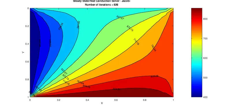
Figure 1: Temperature contour (Solver: Jacobi)
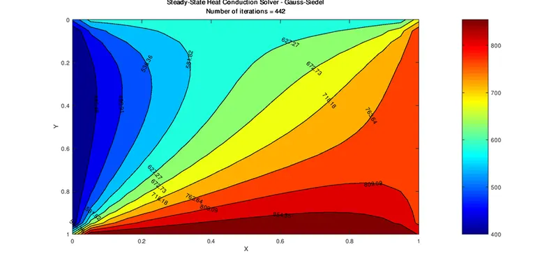
Figure 2: Temperature contour (Solver: Gauss-Siedel)
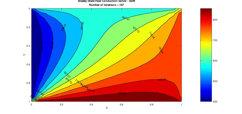
Figure 3: Temperature contour (Solver: SOR)
From the above plots, we would be able to see that SOR method gives faster convergence to results with least number of iterations.
Code for Transient State 2D Heat Conduction equation:
(i) IMPLICIT Scheme:
% 2D transient state heat conduction equation
% Time IMPLICIT method
nx = ny = 20;
x = linspace(0,1,nx);
y = linspace(0,1,ny);
dx = x(2)-x(1);
dy = y(2)-y(1);
T = 300*ones(nx,ny);
T(1,:) = 600;
T(:,1) = 400;
T(nx,:) = 900;
T(:,ny) = 800;
T(1,1) = 500;
T(nx,ny)=850;
T(nx,1) = 650;
T(1,ny) = 700;
Told = T;
T_prev = Told;
dt = 1e-2; %Time step size
tol = 1e-4;
nt = 500; % No. of time steps
alpha = 0.3; % Thermal diffusivity
k1 = (alpha*dt)/(dx^2);
k2 = (alpha*dt)/(dy^2);
w  = 1.5; %Relaxation Factor
method = input('Iterative method = ') %iterative solver selection
if (method==1) %%Jacobi
  jacobi_iter = 1;
  for p = 1:nt
    error = 100;
    while(error>tol)
      for i=2:(nx-1)
        for j=2:(ny-1)
          term1 = ((1+(2*k1)+(2*k2))^-1);
          term2 = term1*k1;
          term3 = term1*k2;
          H = (Told(i-1,j)+Told(i+1,j));
          V = (Told(i,j-1)+Told(i,j+1));
          T(i,j)= ((term1*T_prev(i,j))+(term2*H)+(term3*V));
        endfor
      endfor
  error=max(max(abs(Told-T)));
  Told = T;
  jacobi_iter = jacobi_iter+1;
   end
T_prev = T;
% Plotting the graph
figure(1)
colormap(jet);
A=contourf(x,y,T);
clabel(A);
colorbar;
set(gca,'YDir','reverse');
xlabel('X');
ylabel('Y');
text1 = sprintf('Number of iterations = %d',jacobi_iter);
title({'Transient Heat Conduction implicit Solver - Jacobi';text1});
hold on
pause(0.0001)
end
end

if (method==2) %%Gauss Siedel
  gs_iter = 1;
  for p = 1:nt
    error = 100;
    while(error>tol)
      for i=2:(nx-1)
        for j=2:(ny-1)
          term1 = ((1+(2*k1)+(2*k2))^-1);
          term2 = term1*k1;
          term3 = term1*k2;
          H = (T(i-1,j)+Told(i+1,j));
          V = (T(i,j-1)+Told(i,j+1));
          T(i,j)= ((term1*T_prev(i,j))+(term2*H)+(term3*V));
        endfor
      endfor
  error=max(max(abs(Told-T)));
  Told = T;
  gs_iter = gs_iter+1;
   end
T_prev = T;
% Plotting the graph
figure(1)
colormap(jet);
A=contourf(x,y,T);
clabel(A);
colorbar;
set(gca,'YDir','reverse');
xlabel('X');
ylabel('Y');
text1 = sprintf('Number of iterations = %d',gs_iter);
title({'Transient Heat Conduction implicit Solver - Gauss-Siedel';text1});
hold on
pause(0.0001)
end
end

if (method==3) % SOR Solver
  sor_iter = 1;
  for p = 1:nt
    error = 100;
    while(error>tol)
      for i=2:(nx-1)
        for j=2:(ny-1)
          term1 = ((1+(2*k1)+(2*k2))^-1);
          term2 = term1*k1;
          term3 = term1*k2;
          H = (T(i-1,j)+Told(i+1,j));
          V = (T(i,j-1)+Told(i,j+1));
          T(i,j)= w*((term1*T_prev(i,j))+(term2*H)+(term3*V))+((1-w)*Told(i,j));
        endfor
      endfor
  error=max(max(abs(Told-T)));
  Told = T;
  sor_iter = sor_iter+1;
   end
T_prev = T;
% Plotting the graph
figure(1)
colormap(jet);
A=contourf(x,y,T)
clabel(A);
colorbar;
set(gca,'YDir','reverse');
xlabel('X');
ylabel('Y');
text1 = sprintf('Number of iterations = %d',sor_iter);
title({'Transient Heat Conduction implicit Solver - SOR';text1});
hold on
pause(0.0001)
end
end
PLOTS:
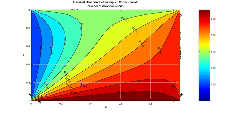
Figure 4: Temperature contour (Solver: Jacobi)
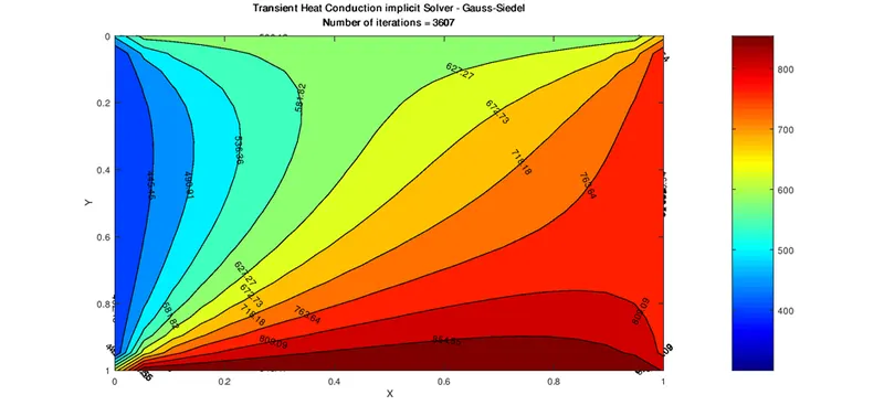
Figure 5: Temperature contour (Solver: Gauss-Siedel)
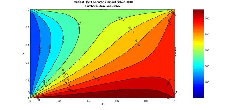
Figure 6: Temperature contour (Solver: SOR)
The same conclusion can be made from the above simulations using different iterative solver as in the case of steady state solution. The SOR methods gave better results with least number of iterations and simulation time as compared to gauss-siedel and jacobi.
(ii) EXPLICIT Scheme:
%2D Transient Heat Conduction solution
%Time Explicit solution
nx = ny = 40;
x = linspace(0,1,nx);
y = linspace(0,1,ny);

% Grid spacing

dx = x(2)-x(1);
dy = y(2)-y(1);

% Initial Temeprature Conditions

T = 300*ones(nx,ny);

% Boundary Conditions

T(1,:) = 600;
T(:,1) = 400;
T(nx,:) = 900;
T(:,ny) = 800;

% Condition at the cornors of the domain

T(1,1) = 500;
T(nx,ny)=850;
T(nx,1) = 650;
T(1,ny) = 700;
Told = T;
dt = 1e-3; %Time step size
tol =1e-4;
nt = 500; % No. of time steps
alpha = 0.3; % Thermal diffusivity for Iron
k1 = (alpha*dt)/(dx^2);
k2 = (alpha*dt)/(dy^2);
method=input('Enter 1 for explicit and 2 for implicit = ')
if(method==1)
 explicit_iter= 1;
 for p = 1:nt
   error=100;
   while(error>tol)
     for i= 2:(nx-1)
      for j=2:(ny-1)
        term1 = k1*(Told(i-1,j)+Told(i+1,j)-(2*Told(i,j)));
        term2 = k2*(Told(i,j-1)+Told(i,j+1)-(2*Told(i,j)));
        T(i,j)= Told(i,j)+(k1*term1)+(k2*term2);
      endfor
    endfor
  Told=T;
  error= max(abs(Told-T));
  explicit_iter=explicit_iter+1;
  end
figure(1)
% Plotting the graph
figure(1)
colormap(jet);
A=contourf(x,y,T);
clabel(A);
colorbar;
set(gca,'YDir','reverse');
xlabel('X');
ylabel('Y');
text1 = sprintf('Number of iterations = %d',explicit_iter);
title({'Transient Heat Conduction Explicit Solver';text1});
hold on
pause(0.0001)
end
end
PLOTS:
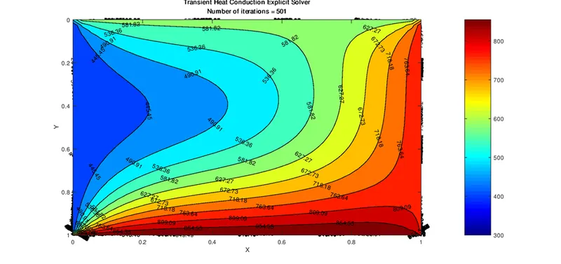
Figure 7: Temperature Contour (Time Explicit Solution)
From the above simulations we can find that, time explicit solution of the PDE is converging faster with least number of solutions as compared to time implicit scheme.
CONCLUSIONS:
- It can be concluded that, among the three point iterative solvers available, i.e., Jacobi, Gauss-siedel and SOR, Successive Over Relaxation method (SOR) yielded, faster convergence for the solution in both the steady state and transient state solutions
- For the transient 2D Heat Conduction solution, explicit method produce better accuracy and less computational time. But the CFL criteria for the time explicit solution must be maintained less than 0.5