Week 5.1 - Mid term project - Solving the steady and unsteady 2D heat conduction problem
AIM: To solve the 2D heat conduction equation using MATLAB for both steady and transient states.
Heat Equation:
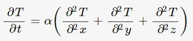
Where T is the function of x,y,z,t and t is "time"
And considering only 'x' and 'y' gives the 2D heat equation.
alpha = thermal diffusivity (assumed as 1.4 )
Assumptions made:
1. The material is homogenous and isotropic
2. Alpha is not the function of temperature
3. The losses like convection loss and radiative loss is been neglected
Solution:
The 2D equation is solved in two different ways;
1. Steady-state (at instant time step)
2. Transient state (including time derivative)
> Various iterative solvers have been used to solve this 2D heat equation such as Jacobi method, gauss seidel method, SOR method.
BOUNDARY CONDITIONS:
T Left = 400K
T Right = 800K
T top = 600K
T Bottom = 900k
The numerical method used to solve this 2D heat equation is the finite difference method(FDM) and considering the first-order approximation for time derivative and second-order derivative for the space derivative terms to get the solution which is as follows,

The above expression is modified to get the solution using different iterative solvers.
CASE 1: Steady-state simulation
Where the solution will be of at the instant time,
CODE:
%steady state heat conduction analysis
clear all
close all
clc

nx = 100;
ny = nx;

L = 1;

x = linspace(0,L,nx);

dx = x(2)-x(1);

y = linspace(0,L,ny);

dy = y(2)-y(1);

T = 300*ones(nx,ny);
T(:,1) = 400;
T(1,:) = 600;
T(:,end) = 800;
T(end,:) = 900;


T_old = T;

cons = ((dx^2)*(dy^2))/(2*((dx^2)+(dy^2)));

tolerance = 1e-4;
error = 1;
iter_method = [1,2,3];

for m = 1:length(iter_method)
% Jacobi method
if iter_method(m) == 1
    iter_name = 'Jacobi method';
    J_iter = 0;
    tic
    while(error>tolerance)
for i = 2:ny-1

    for j = 2:nx-1

        T(i,j) = cons*(((T_old(i-1,j)+T_old(i+1,j))/(dx^2))+((T_old(i,j-1)+T_old(i,j+1))/(dy^2)));

    end

end

error = max(max(abs(T-T_old)));
J_iter = J_iter+1;
T_old = T;

    end
   time = toc;


% Gauss-seidal method
elseif iter_method(m) == 2

    iter_name = 'Gauss Seidel method';
    G_iter = 0;
    tic
    while(error>tolerance)
for i = 2:ny-1

    for j = 2:nx-1

        T(i,j) = cons*(((T(i-1,j)+T_old(i+1,j))/(dx^2))+((T(i,j-1)+T_old(i,j+1))/(dy^2)));

    end

end

error = max(max(abs(T-T_old)));
G_iter = G_iter+1;
T_old = T;

    end
 time = toc;

 %SOR method
 elseif iter_method(m) == 3

     iter_name = 'SOR method';
     omega = 1.4;
    S_iter = 0;
    tic
    while(error>tolerance)
for i = 2:ny-1

    for j = 2:nx-1

        T(i,j) = cons*(((T(i-1,j)+T_old(i+1,j))/(dx^2))+((T(i,j-1)+T_old(i,j+1))/(dy^2)));
        T(i,j) = (T_old(i,j)*(1-omega)) + (omega*T(i,j));
    end

end

error = max(max(abs(T-T_old)));
S_iter = S_iter+1;
T_old = T;

    end
    time = toc;
end
figure(m)
[c,h] = contourf(x,y,T);
clabel(c,h);
colorbar
colormap(jet);
xlabel('Length');
ylabel('Width');
title(iter_name);
ax = gca;
ax.YDir = 'reverse';
end
OUTPUT PLOTS:
> In the steady state there is not any previous time step values to find the solution and hence iterative methods been used to get the solutions.
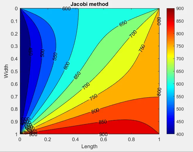
* For jacobi method the number of iterations is very high comparing other solvers as it is updating the temperature values for each and every iterations. And also will take some time to converge.
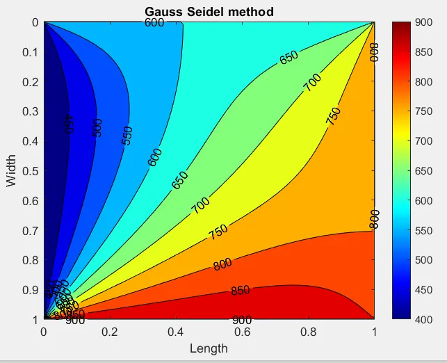
* For Gauss seidel method the number of iterations is high but lower comparing to jacobi solver and it is updating the temperature values then and there which is been known from previous iterations. And also will take lesser time to converge than jacobi method.
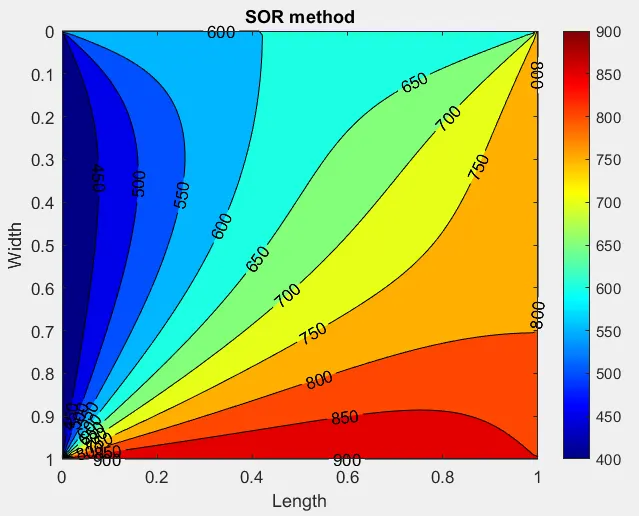
* For SOR method the number of iterations is lower comparing other solvers and it is updating the temperature values then and there which is been known from previous iterations also the factor is been added to make it converge much faster. And also will take lesser time to converge than other methods.
CASE 2: TRANSIENT STATE (EXPLICIT METHOD)
%explicit method
clear all
close all
clc

nx = 100;
ny = nx;

L = 1;

x = linspace(0,L,nx);

dx = x(2)-x(1);

y = linspace(0,L,ny);

dy = y(2)-y(1);

T = 300*ones(nx,ny);
T(:,1) = 400;
T(1,:) = 600;
T(:,end) = 800;
T(end,:) = 900;
dt = 0.14;
t = 1000;
nt = t/dt;
alpha = 1.75e-4;

T_old = T;

CFL = alpha*dt*((1/(dx^2))+(1/(dy^2)));

k1 = alpha*dt/(dx^2);
k2 = alpha*dt/(dy^2);
% tolerance = 1e-4;
% error = 1;
% iter_method = [1,2,3];

% for m = 1:length(iter_method)
% Jacobi method
% iter_method = 1;
% if iter_method == 1
%
     iter = 0;
%     tic
%     while(error>tolerance)
for k = 1:nt
   tic
for i = 2:ny-1

    for j = 2:nx-1

        H = (T_old(i-1,j)-2*T_old(i,j)+ T_old(i+1,j));
        V = (T_old(i,j-1)-2*T_old(i,j)+ T_old(i,j+1));
        T(i,j) = T_old(i,j) + (H*k1) + (V*k2);
%         T(i,j) = cons*(((T_old(i-1,j)+T_old(i+1,j))/(dx^2))+((T_old(i,j-1)+T_old(i,j+1))/(dy^2)));

    end

end

% error = max(max(abs(T-T_old)));
iter = iter+1;
T_old = T;


end
   time = toc;
figure(1)
[c,h] = contourf(x,y,T);
clabel(c,h);
colorbar
colormap(jet);
xlabel('Length');
ylabel('Width');
ax = gca;
ax.YDir = 'reverse';
* For explicit method there are previous iteration values which is been used to find out the next iteration values and so there is only one equation with one unknown which is easy to solve.
OUTPUT PLOT:
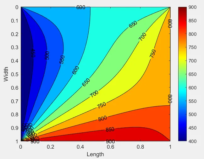
And the explicit method takes much lesser time and iterations for the convergence.
CASE 3: TRANSIENT STATE(IMPLICIT METHOD)
%implicit method
clear all
close all
clc

nx = 100;
ny = nx;

L = 1;

x = linspace(0,L,nx);

dx = x(2)-x(1);

y = linspace(0,L,ny);

dy = y(2)-y(1);

T = 300*ones(nx,ny);
T(:,1) = 400;
T(1,:) = 600;
T(:,end) = 800;
T(end,:) = 900;
dt = 1e-3;
t = 40;
nt = t/dt;
alpha = 1.4;

T_old = T;
T_prev = T;
CFL = alpha*dt*((1/(dx^2))+(1/(dy^2)));
tol = 1e-4;
k1 = alpha*dt/(dx^2);
k2 = alpha*dt/(dy^2);
k3 = 1/(1+(2*k1)+(2*k2));
k4 = k1*k3;
k5 = k2*k3;
% tolerance = 1e-4;
% error = 1;
% iter_method = [1,2,3];

% for m = 1:length(iter_method)
% Jacobi method
% iter_method = 1;
% if iter_method == 1
%
     iter = 0;
     iterative_method = 3;
%     tic
%     while(error>tolerance)
if iterative_method == 1 %jacobi method

for k = 1:nt
  error = 1;


    while(error>tol)

    tic
for i = 2:ny-1

    for j = 2:nx-1


        H = (T_old(i-1,j) + T_old(i+1,j));
        V = (T_old(i,j-1) + T_old(i,j+1));
        T(i,j) = (T_prev(i,j)*k3) + (H*k4) + (V*k5);
%         T(i,j) = cons*(((T_old(i-1,j)+T_old(i+1,j))/(dx^2))+((T_old(i,j-1)+T_old(i,j+1))/(dy^2)));

    end

end
error = max(max(abs(T-T_old)));
% error = max(max(abs(T-T_old)));
iter = iter+1;
T_old = T;


    end
    T_prev = T;
end

elseif iterative_method == 2 %gauss seidal method

 for k = 1:nt
  error = 1;


    while(error>tol)

    tic
for i = 2:ny-1

    for j = 2:nx-1

        H = (T(i-1,j) + T_old(i+1,j));
        V = (T(i,j-1) + T_old(i,j+1));
        T(i,j) = (T_prev(i,j)*k3) + (H*k4) + (V*k5);
%         T(i,j) = cons*(((T_old(i-1,j)+T_old(i+1,j))/(dx^2))+((T_old(i,j-1)+T_old(i,j+1))/(dy^2)));

    end

end
error = max(max(abs(T-T_old)));
% error = max(max(abs(T-T_old)));
iter = iter+1;
T_old = T;


    end
    T_prev = T;
 end

 elseif iterative_method == 3 %SOR

 for k = 1:nt
  error = 1;


    while(error>tol)

    tic
for i = 2:ny-1

    for j = 2:nx-1


        H = (T(i-1,j) + T_old(i+1,j));
        V = (T(i,j-1) + T_old(i,j+1));
        T(i,j) = ((1-alpha)*T_old(i,j)) + alpha*(T_prev(i,j)*k3 + (H*k4) + (V*k5));
%         T(i,j) = cons*(((T_old(i-1,j)+T_old(i+1,j))/(dx^2))+((T_old(i,j-1)+T_old(i,j+1))/(dy^2)));

    end

end
error = max(max(abs(T-T_old)));
% error = max(max(abs(T-T_old)));
iter = iter+1;
T_old = T;


    end
    T_prev = T;
end

end
   time = toc;
figure(1)
[c,h] = contourf(x,y,T,'ShowText','on');
clabel(c,h);
colorbar
colormap(jet);
xlabel('Length');
ylabel('Width');
ax = gca;
ax.YDir = 'reverse';
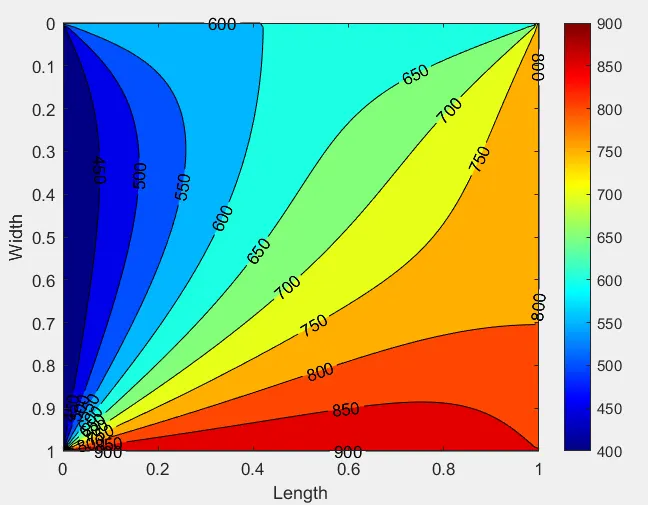
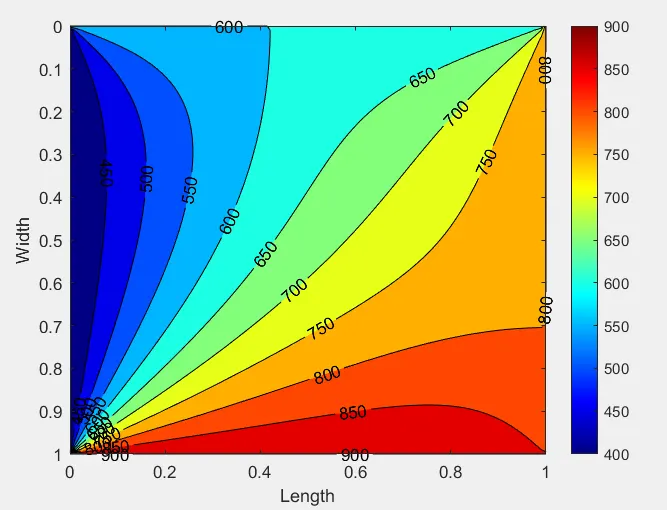
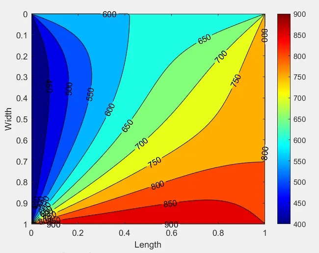
* In implicit method the neighbouring temperature values are been calculated at current time step which makes the process complex and also forming the unknown equations which is been solved by the use of iterative solvers.
OUTPUT PLOTS:
For Jacobi Method:
For Gauss-Seidel method:
For SOR Method:
CONCLUSION:
> So the implicit methods are highly stable than the explicit but it could be a tedious process and so explicit methods are been used.