Week 4- Rolling operation

AIM: - PERFORM A STATIC STRUCTURAL ANALYSIS OF A ROLLING OPERATION.

Objectives:

1. Carry out Static Structural simulation of Rolling operation.

2. Determine:

a) Equivalent Stress for the whole setup.

b) Equivalent Plastic Strain for the workpiece.

c) Directional deformation in Z-axis for the workpiece.

d) Prove that the workpiece has displaced 90 mm.

To begin with the analysis open Ansys Workbench and select the Static Structural analysis from the Analysis Systems.

Double-click on Engineering Data, then go to Engineering Data Sources. Select the

Copper Alloy NL into the project environment.

Now, import the required geometry into the project environment by right-clicking on Geometry and selecting Import, and then browse the file from the location.

Double-click on Geometry to launch the SpaceClaim and load the geometry in it simultaneously.

The geometry will look like this:

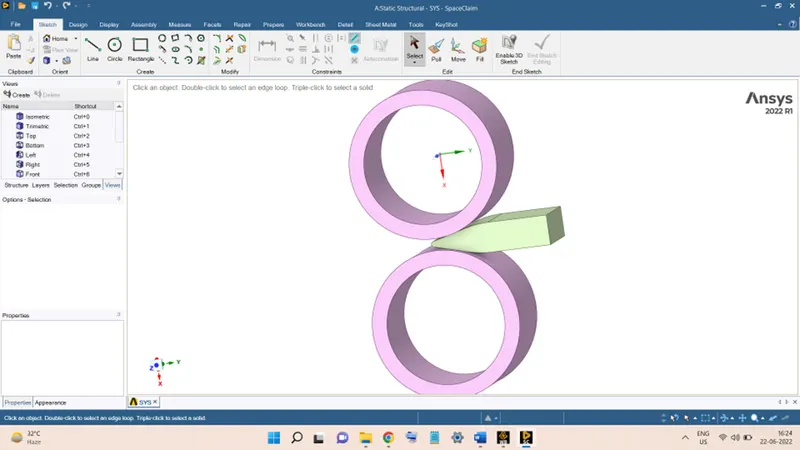
Before moving to analysis some changes are needed to be done in the geometry:

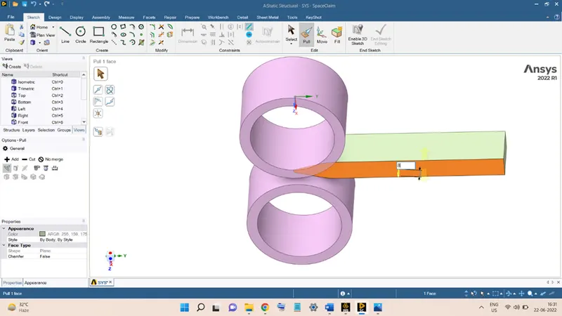
The length of the workpiece is increased by 60 mm. to do this, select the cross-section of the workpiece and go to the command Pull.

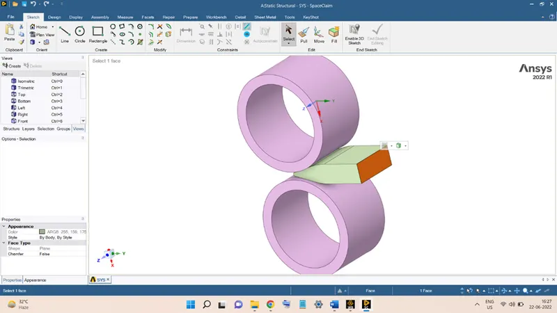
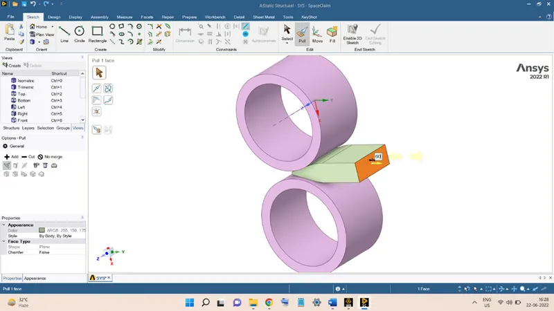
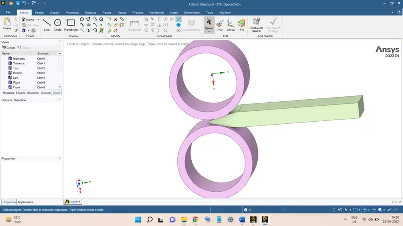
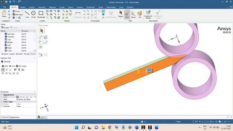
Next is to reduce the width of the workpiece by 8 mm from both sides. This is also done by using the same command.

Select one side face of the workpiece and go to pull command. Now move the cursor in the desired direction. Enter the distance as 8 mm and press Enter to finish. In the same manner do for the other side.

Finally, the geometry will look like this:

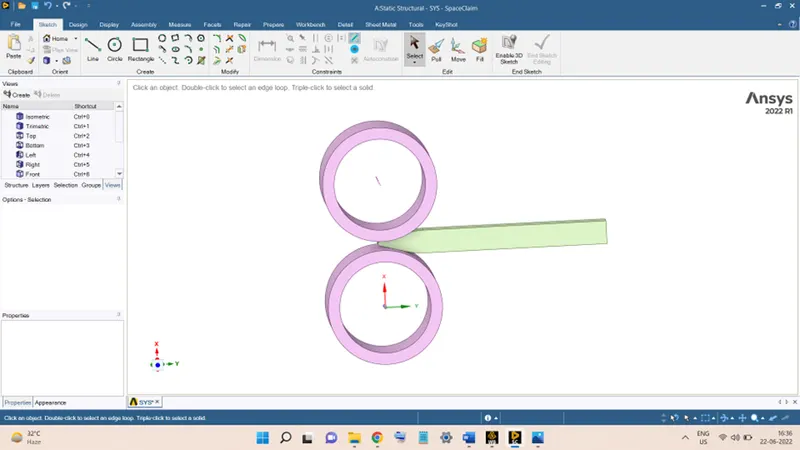
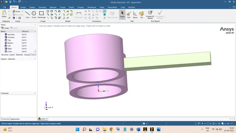
Now the geometry is ready. Right-click on Model and select Edit to launch the Mechanical Module and load the geometry in the module.

The model will look like this:

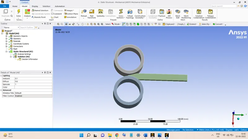
Now, expand the Geometry section and rename the parts of the geometry as shown below:

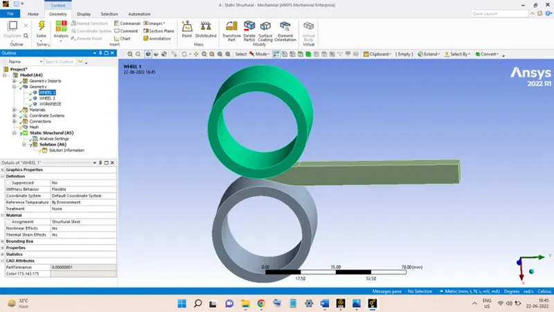
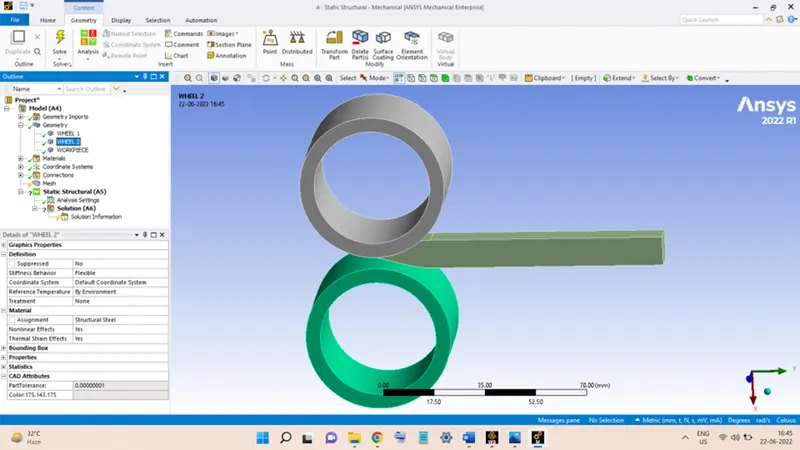
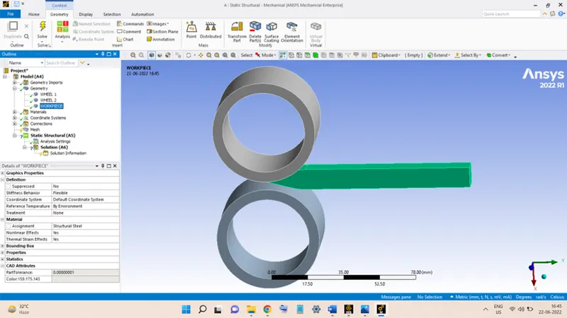
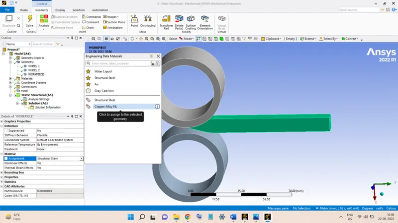
For the WORKPIECE, go to the Material section and change the Assignment to Copper Alloy NL.

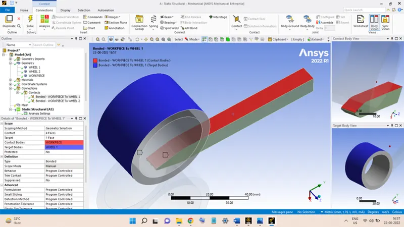
Next, go to the Connections section and expand the Contacts. Select the two pre-assigned contact regions and Flip them by right-clicking and selecting the Flip option. Then, again right-click and select Rename Based on Definition.

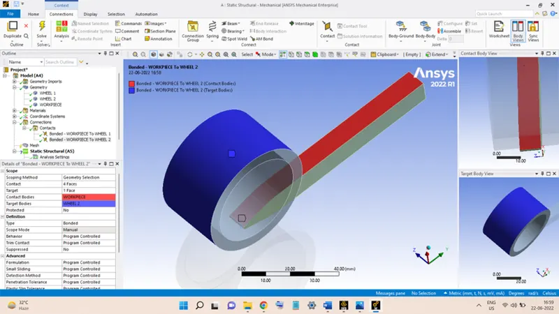
Next, select the first contact region and select all the remaining Top surfaces of the WHEEL 1 under Target and click Apply. Then, select all the portions of the top surface of the WORKPIECE under the Contact section and click Apply. The contact will now be looking like this:

Do the same for the second contact region also.

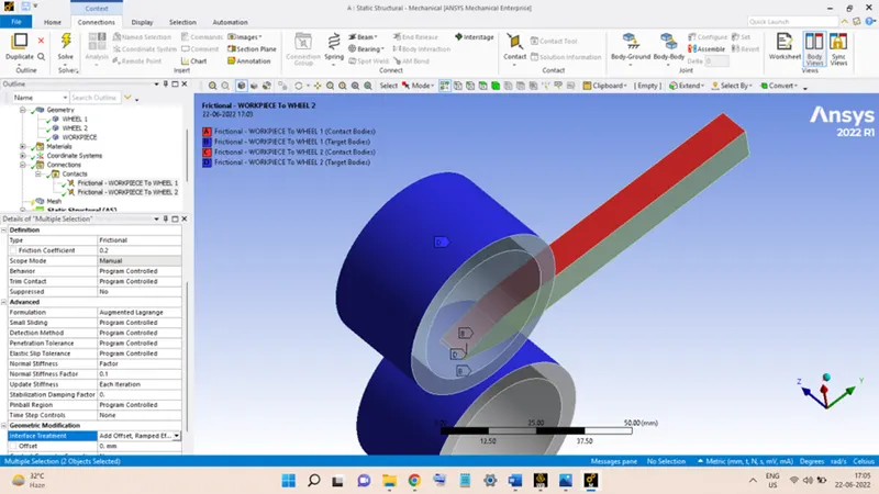
Now, select both the contact regions and perform the following changes:

In the Definition section, change the Type to Frictional and enter the value of Friction Coefficient as 0.2.

In the Advanced section, keep the Formulation as Augmented Lagrange.

Normal Stiffness as Factor and value of Normal Stiffness Factor as 0.1, keep Update Stiffness as Each Iteration.

In the Geometric Modification section, change the Interface Treatment to Add Offset, Ramped Effects.

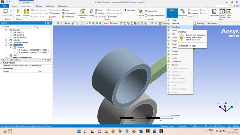
Now, the joints of the rollers are to be added to the geometry. To do this, right-click on the Connections section. Click on Body-Ground and select the Cylindrical.

Now, select the inner surface of the WHEEL 1 and hit Apply.

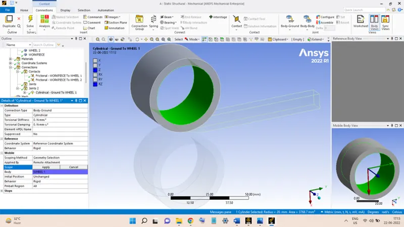
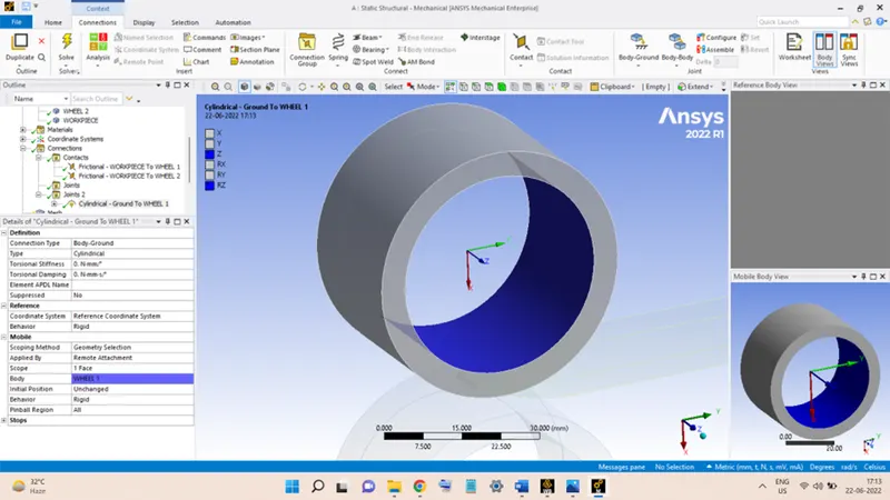
Check for the Z-Axis of the joint must point inwards, if not, then go to the Reference section and click on Reference Coordinate System and select the Z-axis in the model and flip its direction and hit Apply.

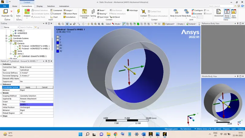
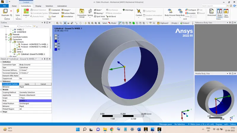
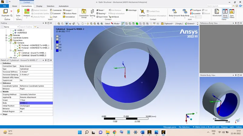
Perform the same to add the Cylindrical joint for the WHEEL 2.

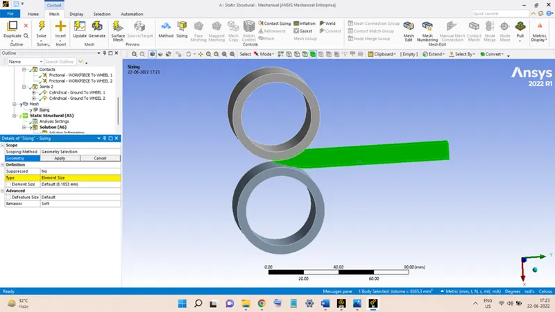
The next step is to mesh the geometry. For this, right-click on the Mesh section, go to Insert and select the Sizing option. Select the WORKPIECE whole as a body and click on Apply. Then, enter the Element Size as 2 mm.

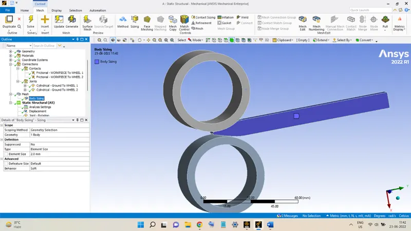
Now, right-click and select Generate Mesh option to mesh the geometry. The model after meshing will look like this:

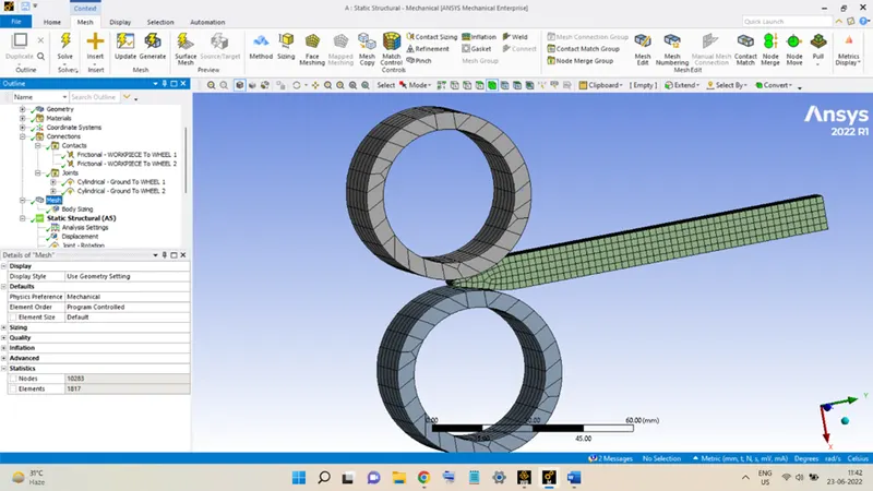
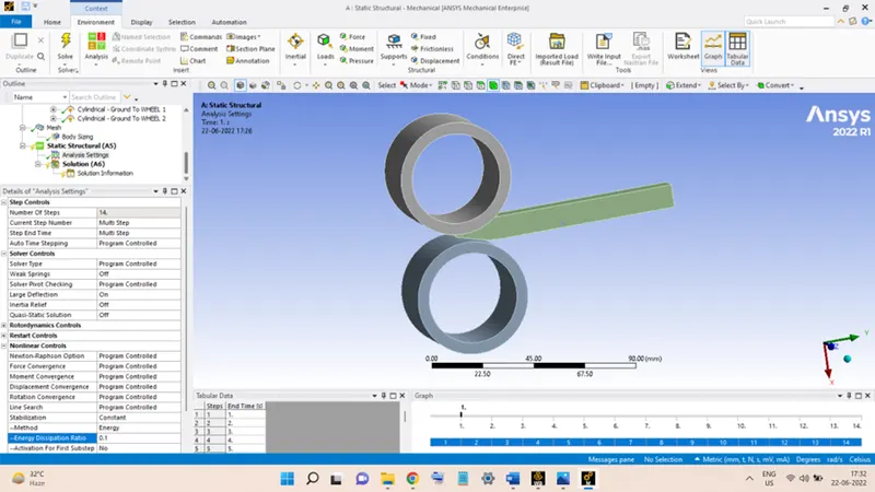
Next is to supply the analysis settings to the model. In the Analysis Settings section go to the Step Controls section and set the Number of Steps as 14. Select all the 14 steps and in the Solver Controls section turn the Large Deflection ON. In Nonlinear Controls set the Stabilization to Constant and set the value of the Energy dissipation Ratio as 0.1.

Now, the Joint loads and displacements are to be assigned to the model.

Add Displacement to the WORKPIECE:

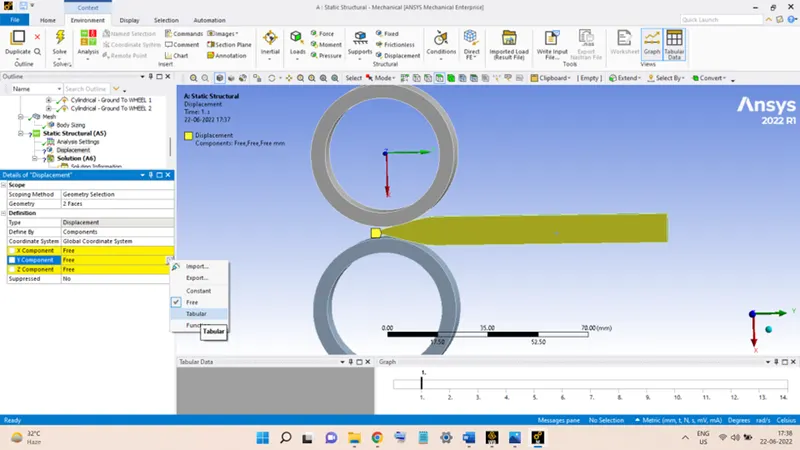
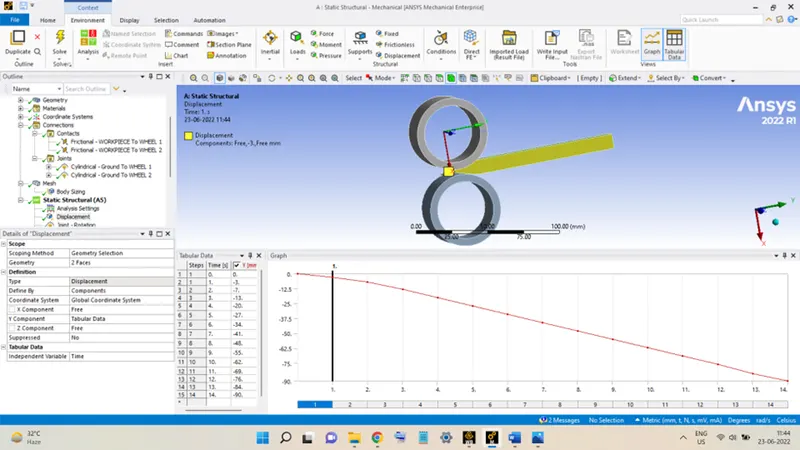
The WORKPIECE will be given a 90 mm displacement into the two rollers along the Y-Direction. To do so, right-click on Analysis Settings, go to Insert, and select the Displacement. Select the BOTH SURFACES of the WORKPIECE, as shown in the figure below, and click Apply.

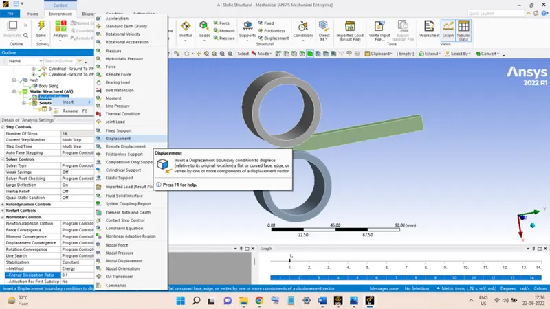
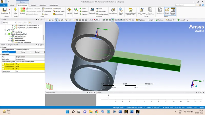
Then select the Y-component and set it as Tabular. Now enter the values from 0 to 90 mm in the table.

Add Rotation to the Wheels:

Right-click on Analysis Settings, go to Insert, and select Joint Load.

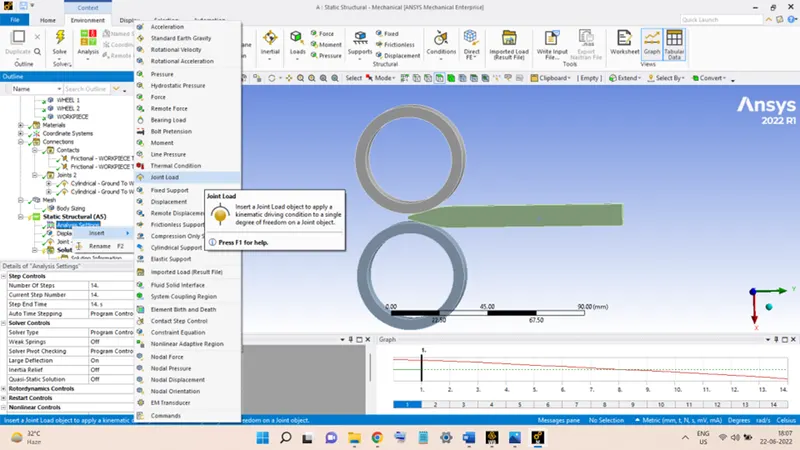
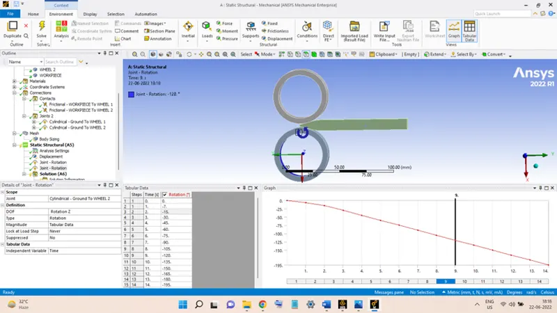
In the Scope section, select the WHEEL 1 joint first. In the Definition section, click on DOF and select Rotation Z, in Type select Rotation and Magnitude select Tabular Data and enter the values in the table as follows:

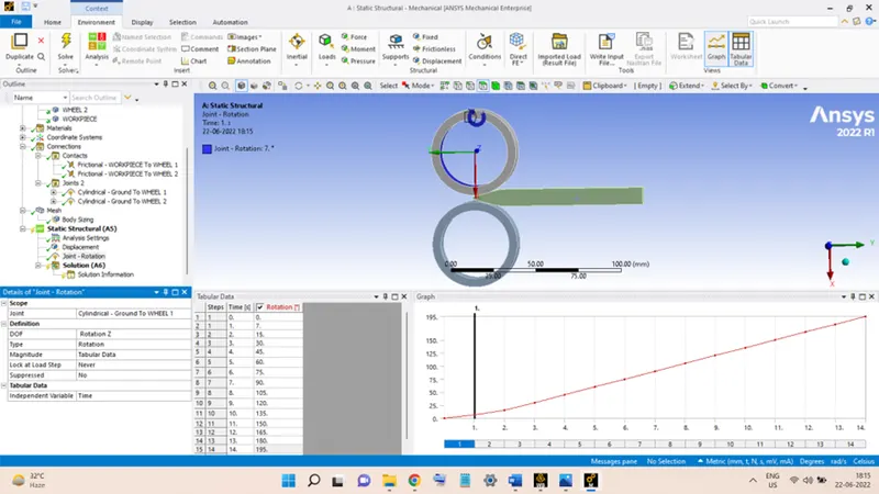
Similarly, do the same for the WHEEL 2 and angles should be entered with a negative sign, as shown below:

With this, the model is ready for analysis. Before starting the analysis the required output result parameters are added to the analysis.

To add the output parameters, right-click on Solutions and go to the Insert and select Stress and then select Equivalent (Von-Mises).

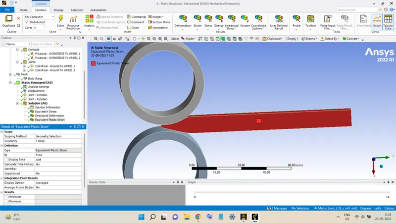
Similarly, add the Equivalent Plastic Strain and in the Scope section, click on Geometry, select only the WORKPIECE body, and hit Apply.

Now add the Directional Deformation and go to Geometry and select the two opposite faces of the WORKPIECE and hit Apply. Set the Orientation to be Z-Axis.

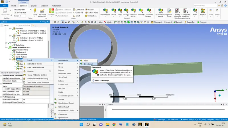
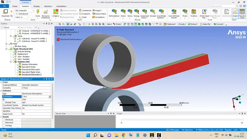
Again, select the Directional deformation and this time add the two front faces of the WORKPIECE and hit Apply, and set the Orientation to be Y-Axis. This result will help in determining the actual distance moved by the WORKPIECE during the rolling operation.

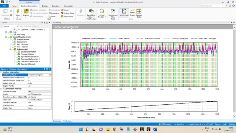
Now, click on Solve to begin the analysis. After the analysis is completed successfully, the Force Convergence graph is shown below:

RESULTS:

Equivalent Stress:

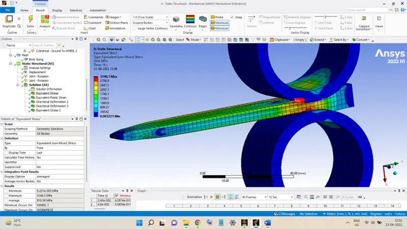
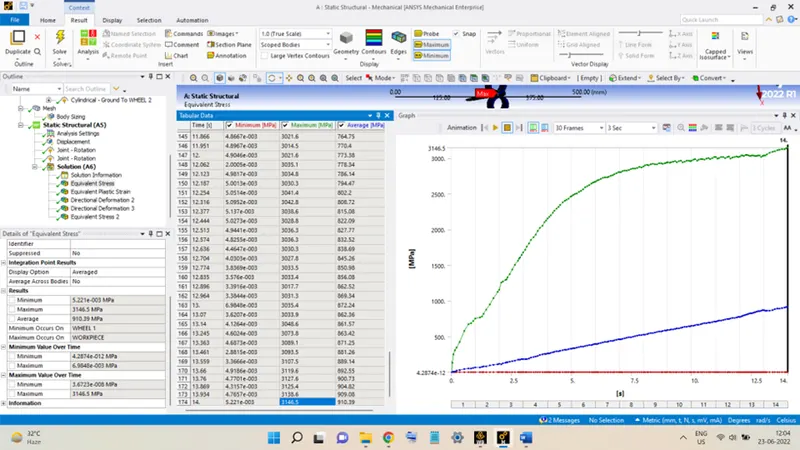
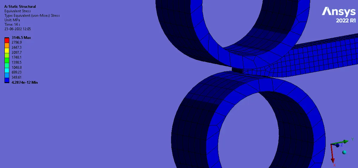
The above figures show the variation of the stress developed in the setup during the rolling operation. it shows that the maximum value of the stress reaches up to 3146.5 MPa during the operation.

Equivalent Plastic Strain:

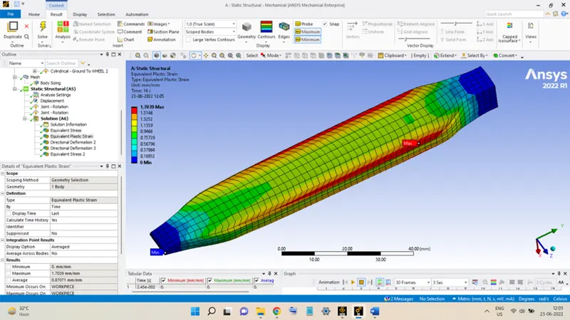
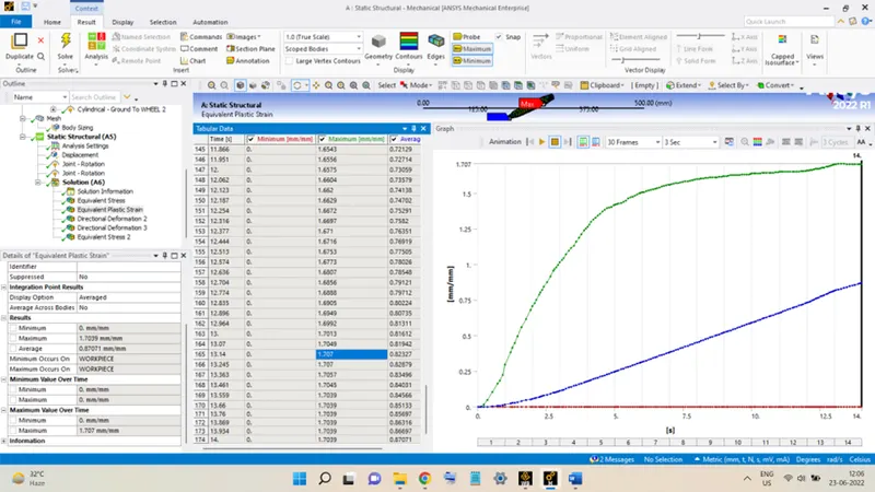
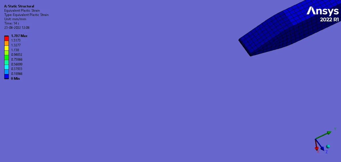
The above figures show how the Plastic Strain is developed in the WORKPIECE and its variation during the operation. Plastic Strain attains a maximum value of 1.707 as shown above.

Deformation of WORKPIECE in Z-direction:

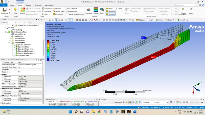
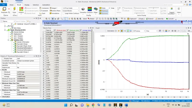
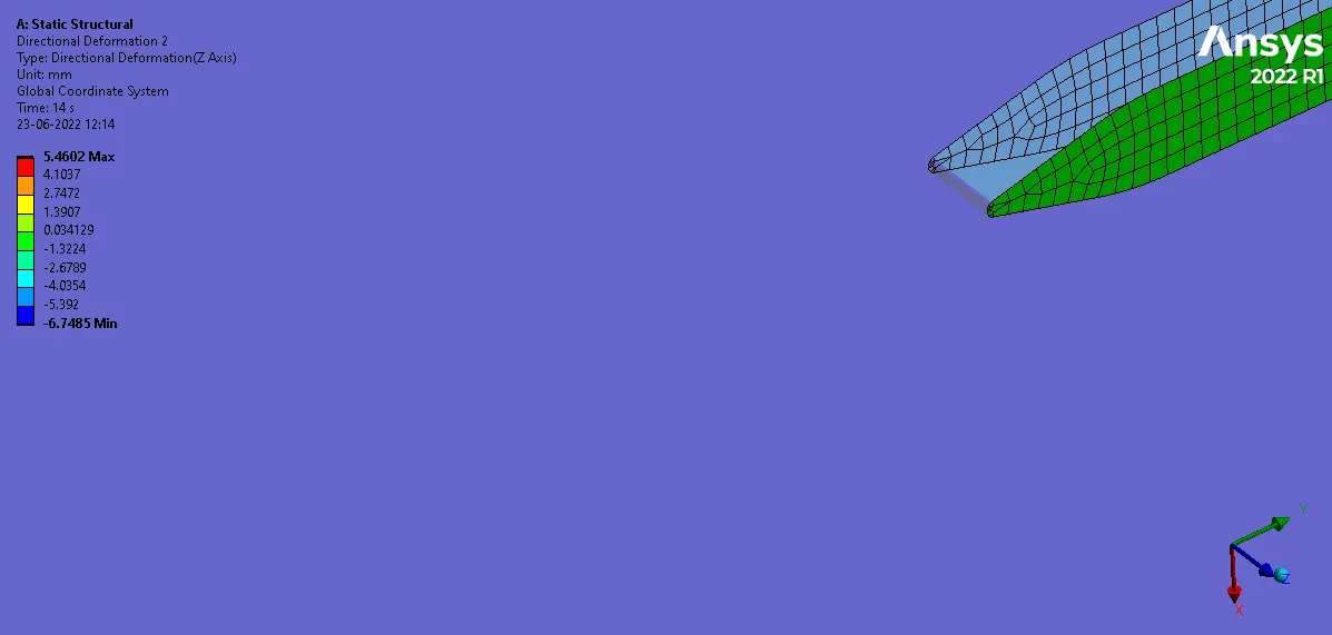
The above figure shows the deformation of the WORKPIECE along the Z-Axis during the rolling operation. Both the faces have different values for the maximum deformation. The one face Is having maximum deformation of 5.4397 mm and at the other face, it is -6.7485 mm (negative sign implying deformed in negative Z-direction).

Deformation of the WORKPIECE in Y-Direction:

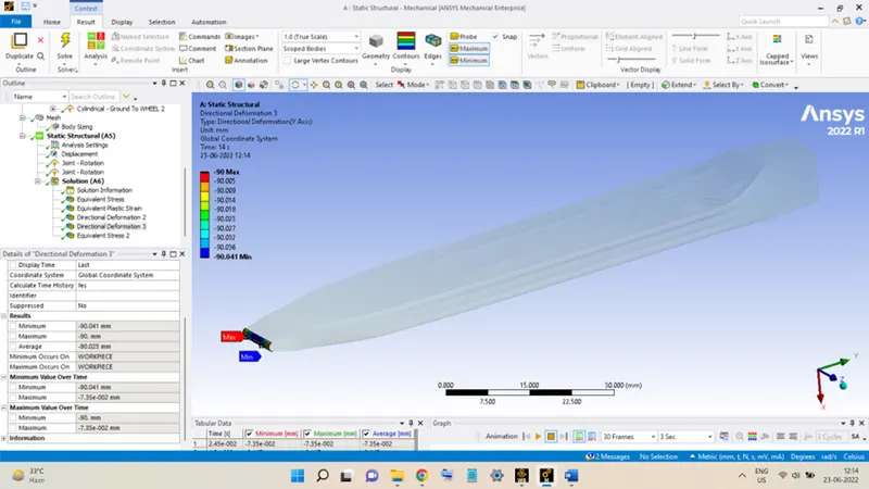
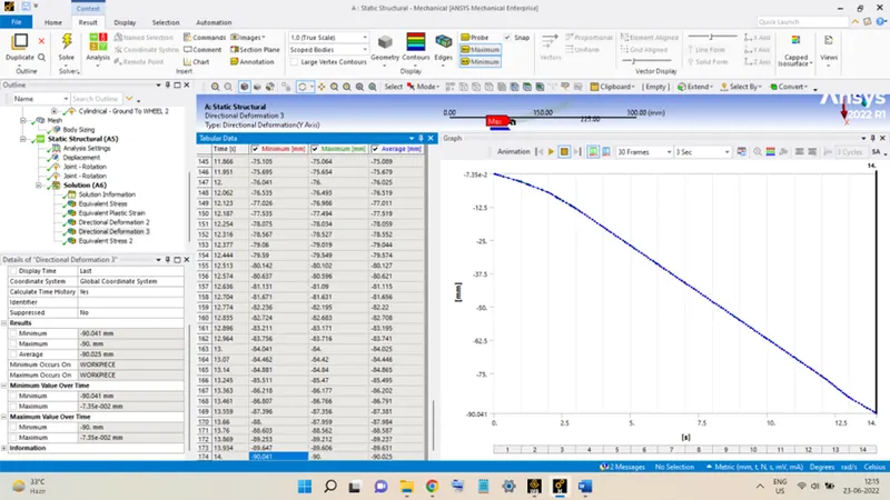
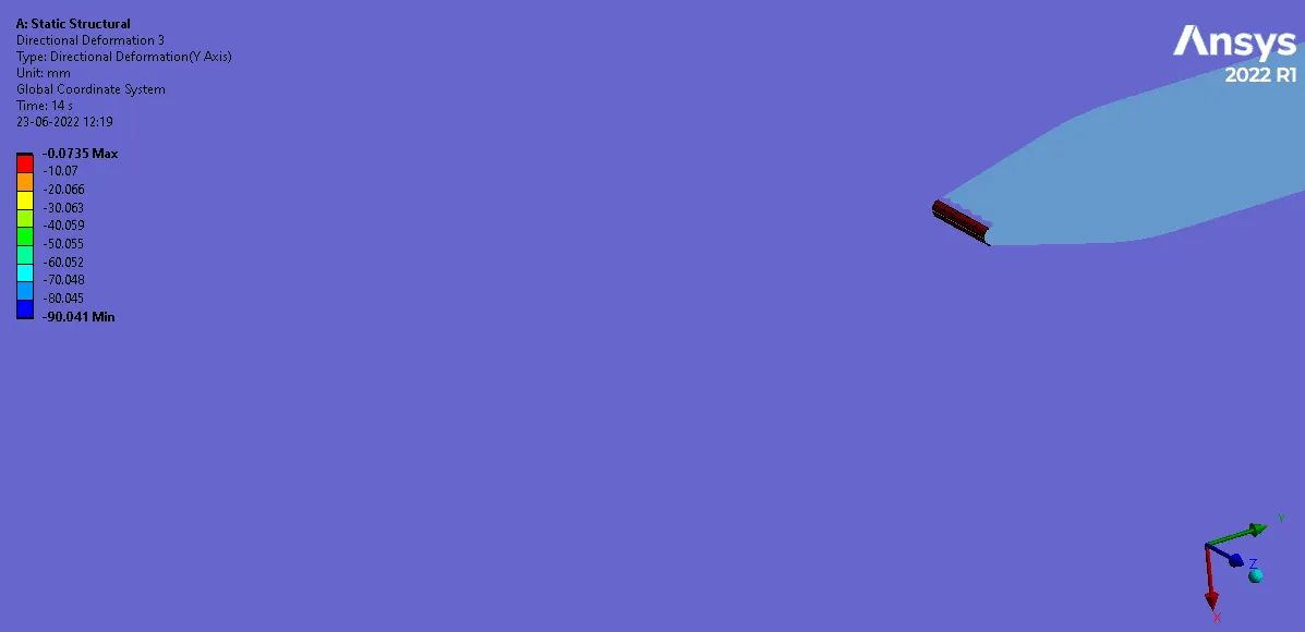
The above figures show the distance traveled by the WORKPIECE during the rolling process. As can be seen in the graph, the maximum deformation is equal to 90.041 mm along the negative Y-Direction. thus, it can be safely said that the WORKPIECE traveled a distance of 90 mm during the operation.

Stress in WHEEL:

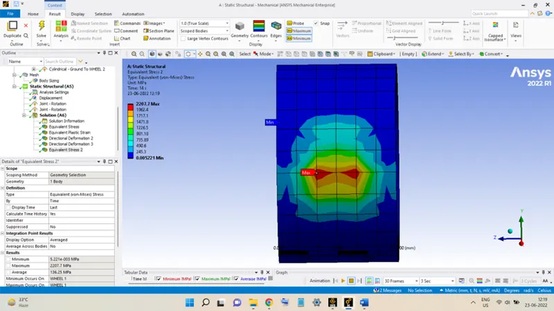
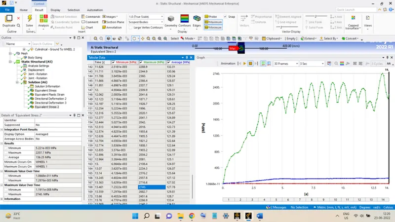
The above figure shows the variation of the stresses developed in the WHEEL during the rolling operation.