Transient flow simulation in a channel with mobile throttle body
OBJECTIVE:
Setup and run transient state simulation for flow over a throttle body.
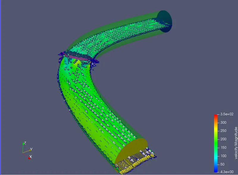
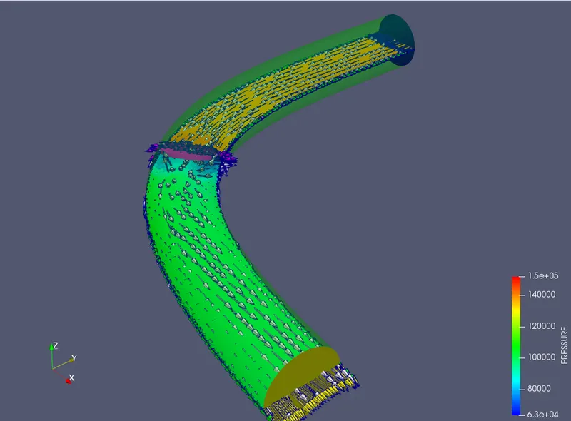
Post process the results and show pressure and velocity contours.
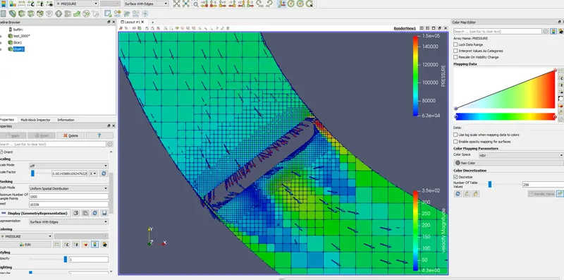
Show the mesh (i.e surface with edges)
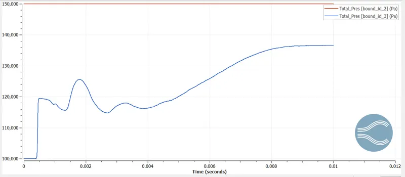
Show the plots for pressure, velocity, mass flow rate and total cell count.
Also show the calculations on how you calculated an end time for the simulation.
Create an animation in which it throttle movement should be visible.
- Upload an animation on You tube and provide the You tube link for an animation in your report.
Theory:
Here we have a .STL file of an elbow pipe body where we simulate the 2 types of flow. Steady-state flow and transient flow. In steady-state we have the profile quite smooth just like the previous flows we did in backward flow and flow over the box where there was not any turbulence but a general flow simulation was done. However, the flow is similar to previous flows but it has one more system inside the profile called the Throttle body. Now typically, in real-time, the Throttle body plays a vital role in metering the airflow. It controls the airflow rate through the flow area by the throttle valve. The airflow through the throttle body increase when increasing the throttle valve opening positions. In this case, there's no valve here.
So the objective is to perform a steady flow simulation with the throttle body inside which is fixed and is independent of the flow. There will turbulence flow at the region where the throttle body is. we need to monitor every parameter while the floe is going.
Case Setup:
Now here we start by running the COnverge CFD software were building up a case setup of channel flow that represents the parameters to run the data. No where we already have a .STL file so we download it grab the file and drag it to the converge or you can do with the conventional method by opening new projects in the new section. But here we have this elbow block.
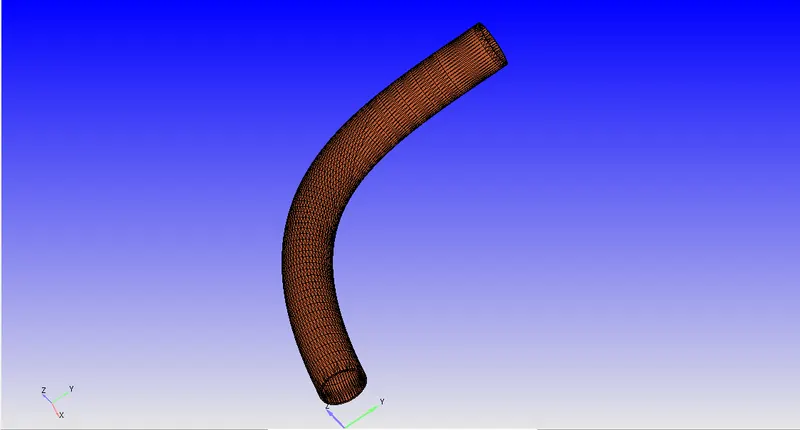
ofcourse with some thickness to it, which is not of interest as we are not doing any conjugate heat transfer where we perform thermodynamic analysis. Here we are about to analyse steady state flow and we need no thickness with fully closed surface with no open edges.
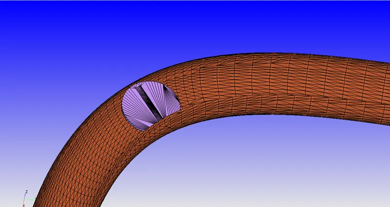
and that is why we are gonna use tools like REPAIR to delete the unrequited thickness by angle and by open edges tools to make it look elbow Channel with no thickness. which should look like this.
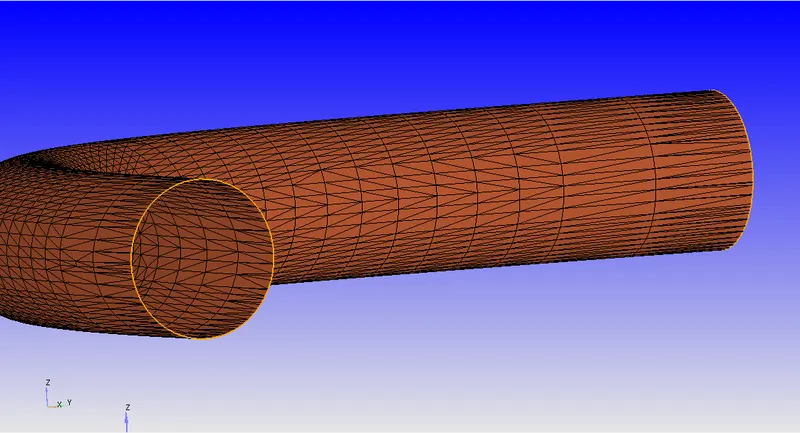
we do have to eliminate the thikness of the block to get it to look like above image. As you can see there are two open edges we can fill it up with PATCH tool to make it the closed channel. You can also toggle the NOMALS to view the normals on the geometry to view the flow motions.
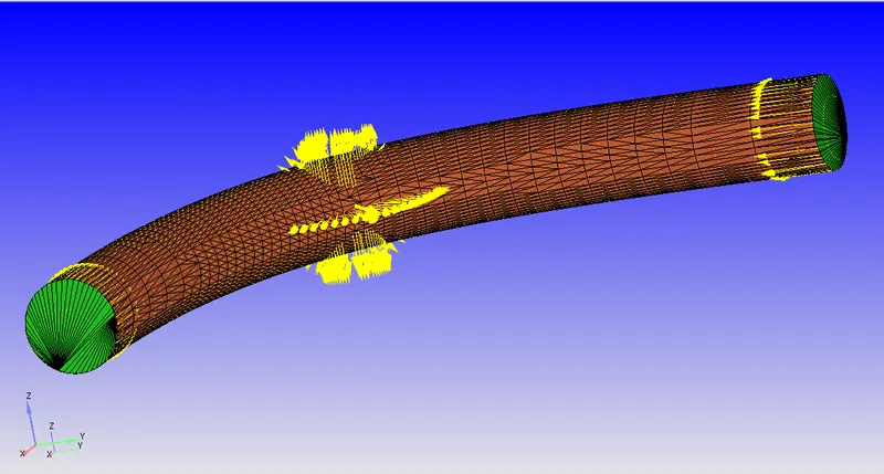
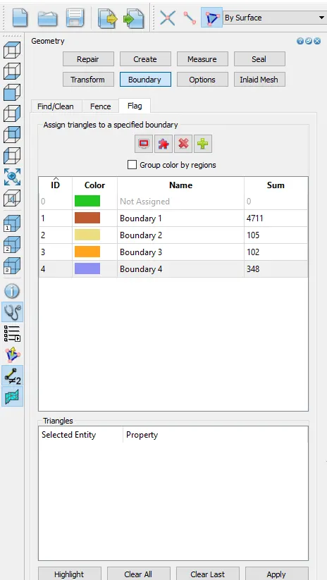
Now that we have geometry set along with boundaries to be assigned as INLET, OUTLET, ELBOW-WALLS, we can forward for the case setup now. Now the Assigning all types of Technical parameters for the flow property to case set up in the bottom right side. Below is the image is shown where all the case setup should like. The green tick indicates the all the parameter is set right according to flow properties. NOTE that it has THROTTLE BODY inside of it which is considerably static throughout the analysis. We can view this as below.
Assigning the boundaries is must so that converge can recognize which is which to begin and understand the case setup part.
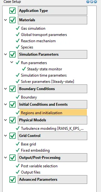
Before Jumping into the simulation part in Cygwin, one needs to set up the parameters in case set up to look like the above image. The value represents in the above image shows the completion of the properties, here's how every section needs to be done.
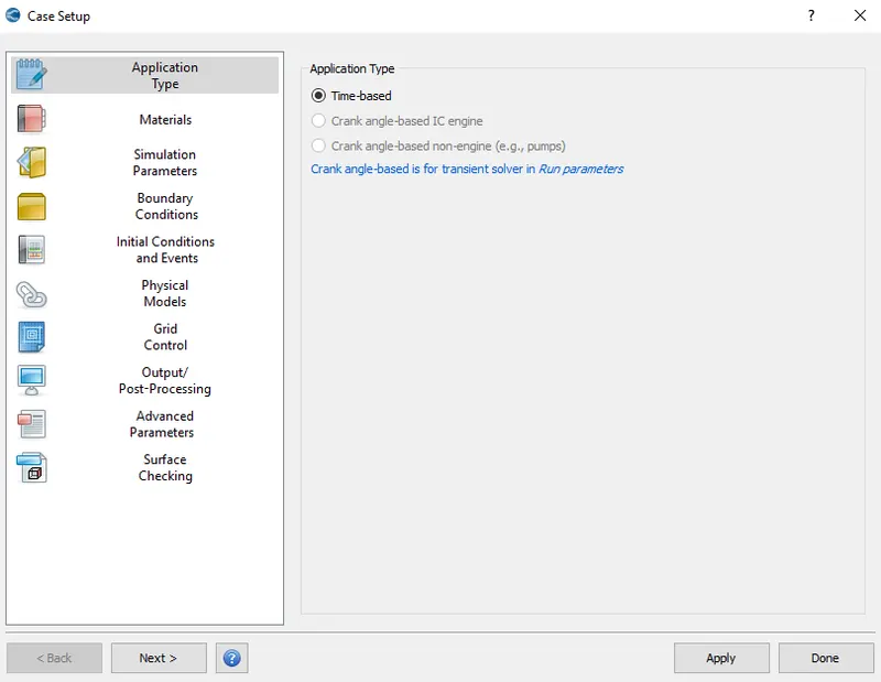
Application type:
Selecting the Time-Based is the option available here as we are only setting up a simple channel flow profile, to begin with.
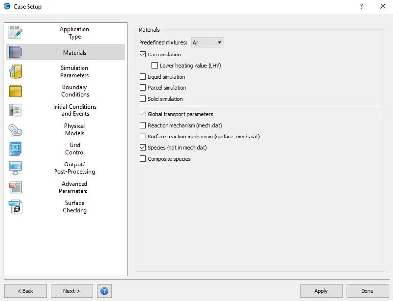
Materials:
By selecting the predefined Mixture as AIR and checking Species.dat and gas simulation we complete materials setup.
Moving on to another section we have SPECIES where we O2 and N2 in the gas.
Moving on to Another section called Run Parameters where we assign very important terms to proceed.
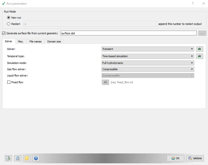
We select steady-state solver in the solver section and Full hydrodynamics in the solver section because we are going for simple channel flow. Where there is no complication in this system technically. The full hydrodynamic always take a lot of time to process the data files as it runs the basic Navier stokes equation through and through which might take a lot of time. Hydrodynamics would be a viable option here but again the fluid dynamics properties won't take place while running which is also not quite an option in some cases. SInce it's a simple flow Full hydrodynamics option can fully be considered and no complications would be three.
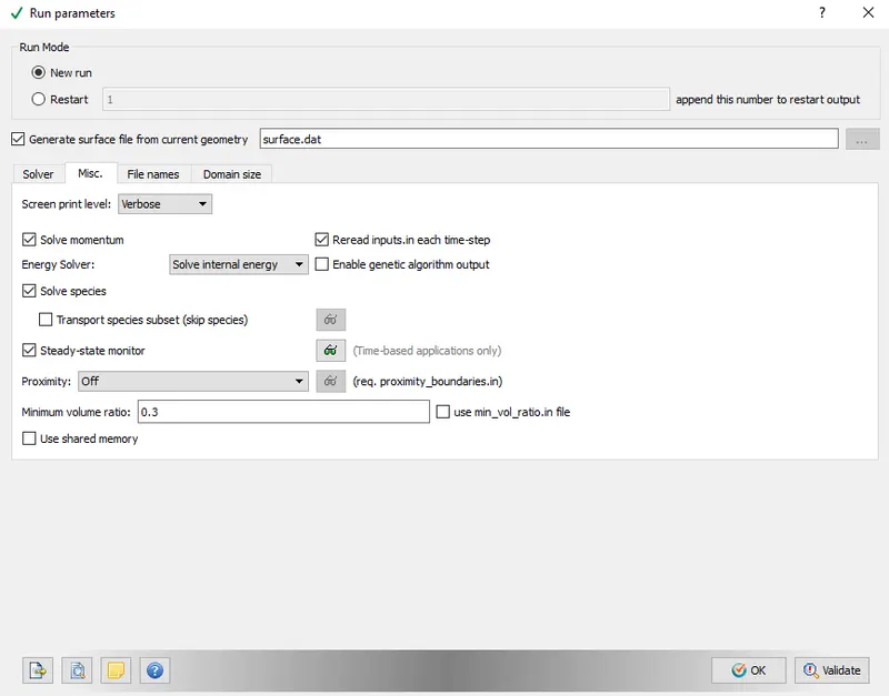
Followed by Solver we have the Misc. option where we select the steady-state here again including unchecking the used memory option as we don't want extra storage for the simulation.
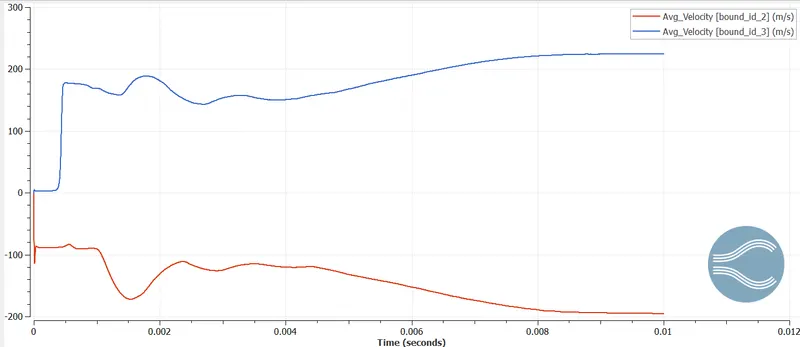
Moving onto the steady-state monitor we have a list selecting section where we ADD first and then select Avg velocity. Now, this is the section where we need those parameters that we need to display when getting the output. So here we need to know the avg velocity of the flow when it flows out of the channel in OUTLET. That's is why assigning the value to the parameter.
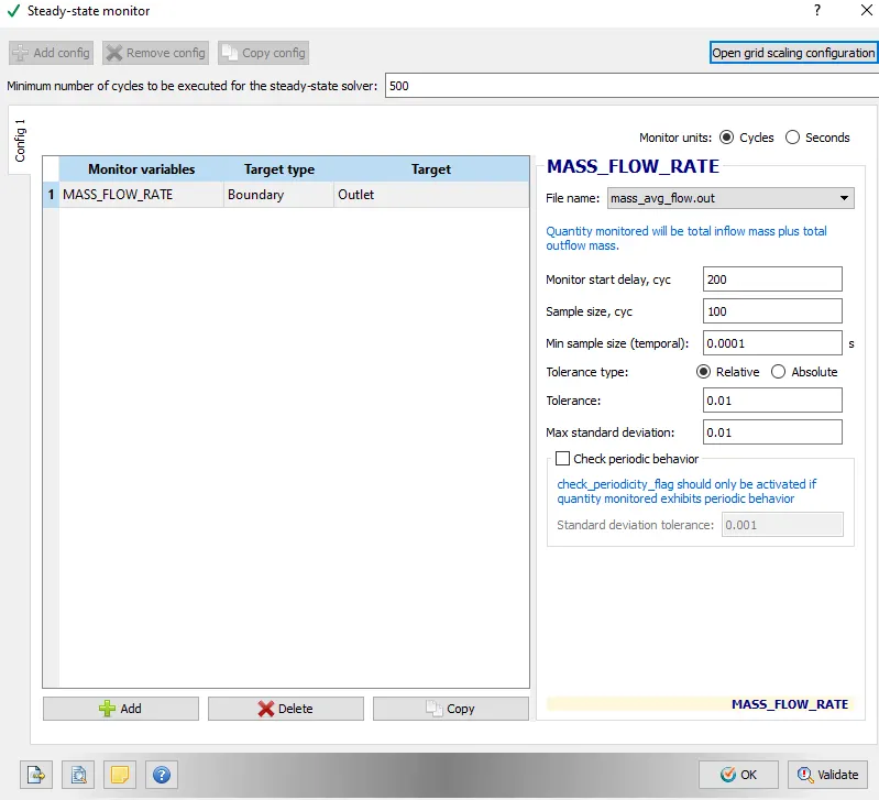
Assigning the value and validating it and Ok.
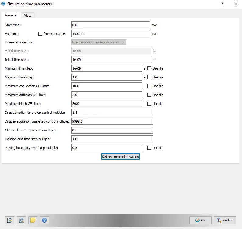
In another section called Simulation-Time Parametres here, we have all the values that are going to be involved in the simulation we are setting up.
The values here as follows for assigning. The end time is always 15000.
In the nest section of Solver-Parameters, we have what kind type of Navier-stokes solver, which is a Pressure-based solver for this flow.
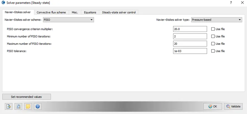
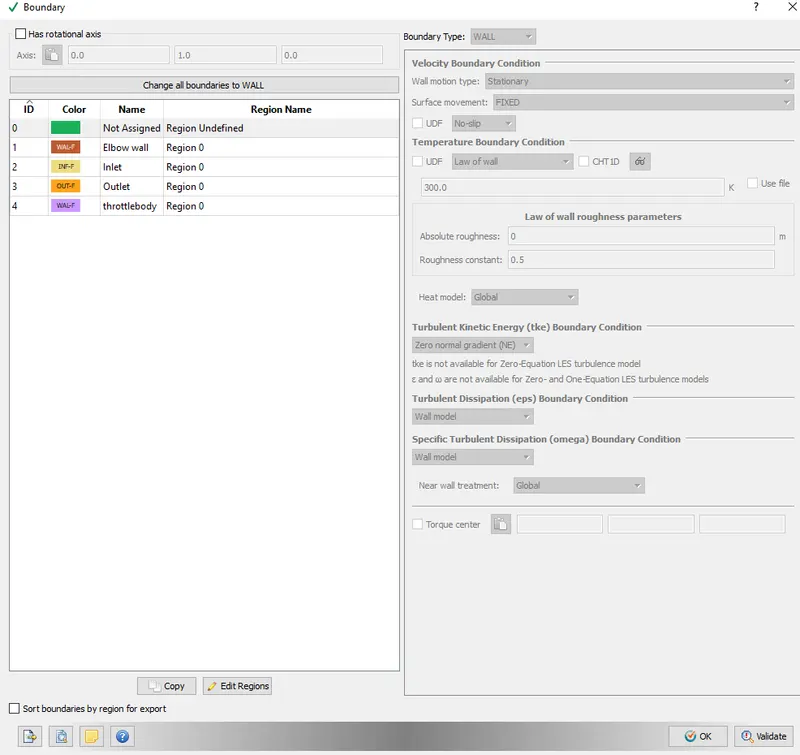
The next section is really important as we assign the Boundary condition for the flow and the walls around it to define the type of fluid flow effect on it while flowing.
INLET - Region 0
OUTLET - Region 0
ELBOW-WALLS - Region 0
THROTTLEBODY- Region 0
above is how we assign the properties along with section-wise with INLET PRESSURE 150000.0 Pa and OUTLET PRESSURE 100000.0 Pa with 300K temperature in temperature boundary conditions.
In case of Transient flow:
Since there's a transient flow throughout the system we have to provide a different input setup for THROTTLE BODY in BOUNDARY,
Here we have to define the axis of rotation and center of rotation values so while in the simulation the throttle body moves to make it the transient flow with turbulence around the body boundary. These are the values we have here.
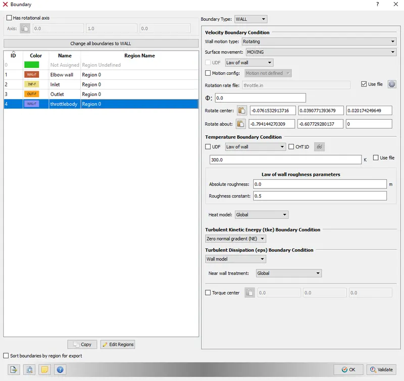
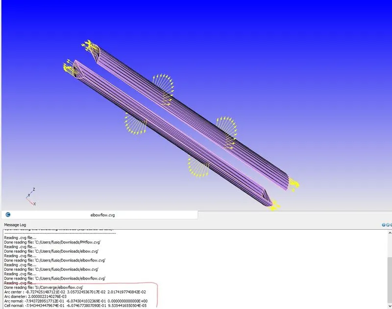
Here the value of rotation and rotation about can be taken from the geometry itself by using MEASURE tool
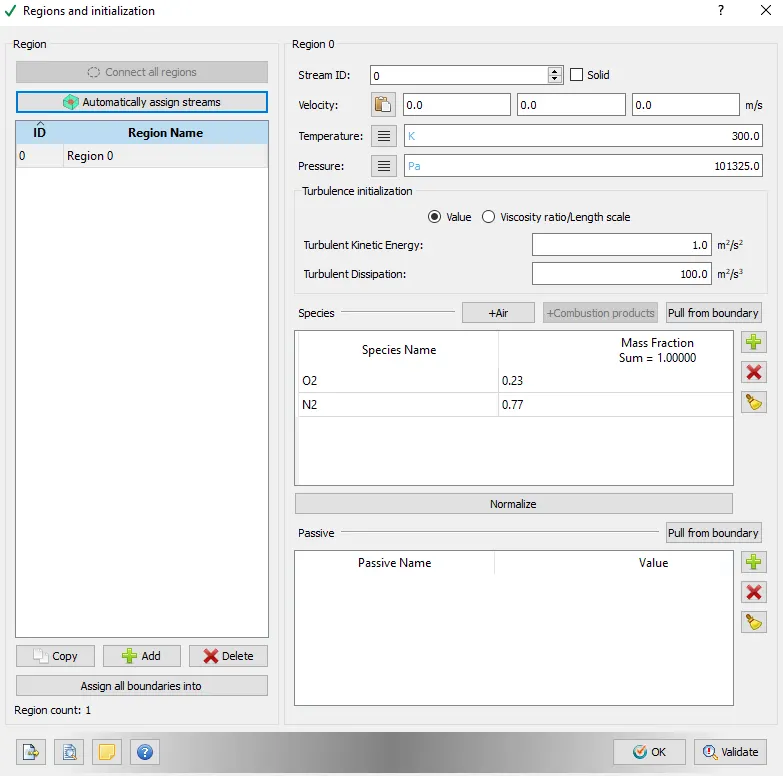
In the Region and Initialization, We need to add the O2 and N2 ratios for the flow.
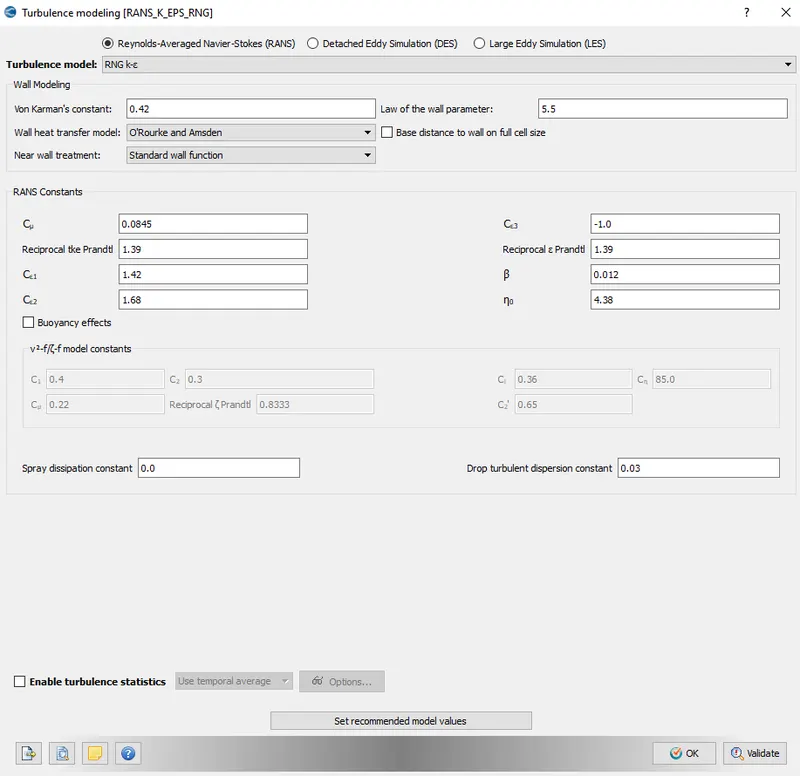
IN the Physical-Modelling We need to check the turbulence modeling as there will be turbulent flow over a channel because of the throttle body. We select the RNG k e method to solve the analysis.
Now the next section is Base Grid, where we assign the INPUT coordinated for the channel so that it has a different output for different inputs. This where the box we create in the first stem gets its own assigned values of coordinates in a cartesian lane.
- dx = 4e-3m, dy = 4e-3m, dz = 4e-3m
Next is Output files where the simulation through data files per cycle is determined. The timings per cycle here is really important as it shows the data files per cycle which are required to tun the smooth curve simulation and animation in ParaView. These are the input data that needs to be assigned here as below.
So here your wholes case setup is READY and we can proceed with Post process simulation in CYGWIN. After completing the simulation in Cygwin and post process 3D output files in PARAVIEW we get the below view with the surface with edges.
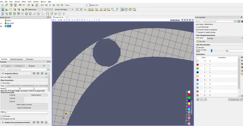 -------> Case 1
Now here is the unaccomplished part, we have the mesh ready at the surface of the channel however we the refinement is not good though the flow is possible on INLET and OUTLET, although the region around the throttle body is messy. As the flow continuity is unrealistic, the box on the surface determines flow probability making it possible flow. around the throttle body there ain't much of box or mesh to produce smooth flow.
However, we can create a possible mesh around a particular region that accelerates the fluid flow. We need a local mesh refining tool to undo the possibility of flow. So we have a tool called FIXED EMBEDDING in case setup under the grid controlling section. where we add embedding at the throttle boundary to the scale where we get smooth couple of mesh. this where we can find fixed embedding.
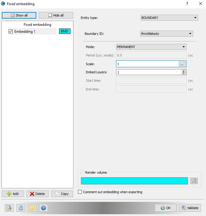
After inputting values, which is we are putting boundary as throttle body on the permanent mode, we get the difference in refinement near the boundary of the throttle body. the result is below in ParaView after converting the 3d output data files in post-processing scenario.
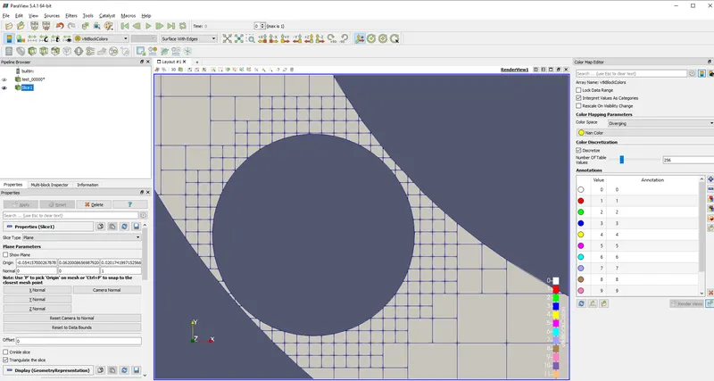
As here you can see that the refinement is quite fine which makes the flow more feasible than before we had no refinement at all. This does make a lot of difference here. Although we still have a problem with the upper wall on the throttle body for this pic it may situate on the left boundary. We can see there isn't much if vivid mesh around the region. We can always go for the LOCAL EMBEDDING again but to try a different approach here we can minimize the BASE MESH GRID which will make the mesh small and inturn the refinement finer. So in this case again we can go
dx = 2e-3m, dy = 2e-3m, dz = 2e-3m with scale 3 and layer 2 o the FIXED EMBEDDING method. the following is the desired mesh contour of channel.
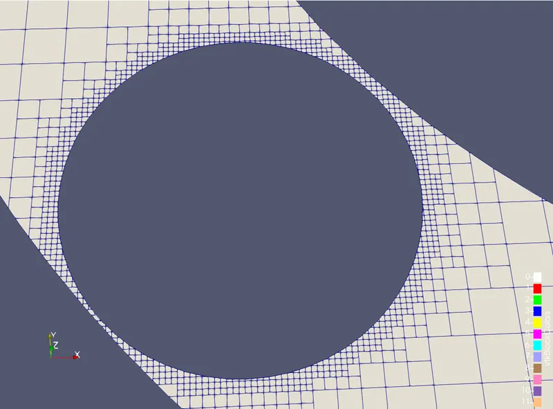
Much more smoother much more refined at the edges and boundary of the throttle body. However getting your base mesh grid lower and local embedding larger doesn't make your mesh great as at on point it's gonna crash the whole profile, It should be just the amount that the flow takes place feasible.
Post-Process Simulation (CYGWIN):
Run Cygwin go to the directory where we have our basic .dat files in the converge folder. These are the following commands in Cygwin to go to the directory
$ cd
and tun the following command to convert,dat files into 3d OUtput dat files.
$ mpiexec.exe -n 2 "the path where you have intelmpi.exe" restricted </dev/null> logfile &

This was how-to convert .dat files into 3d Output data files for post-processing.
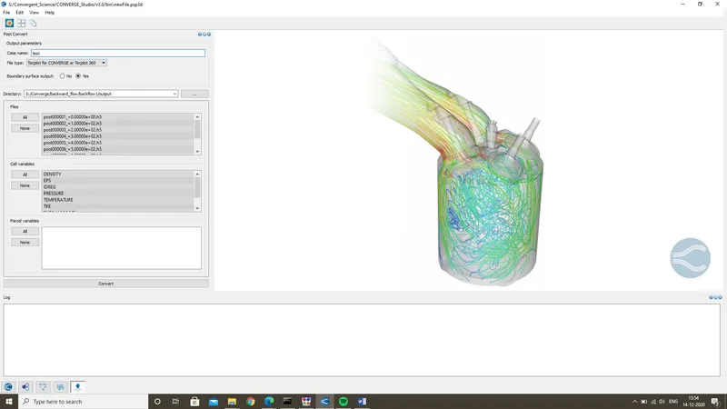
after that, we need to convert those files so that ParaView can read it 3d output files. We need to do through Cygwin to convert those files too with the following command or we can proceed with the converge itself as it provides nice feature to post convert 3D files to DAT files which Paraview can read. Here we need to name it as test and go to the directory of OUTPUT folder where all the files dumped and select ALL and CONVERT just like image shown below. and for post-processing the DAT and files we can directly convert it from CONVERGE as below.
OUTPUT:
Velocity Contour:
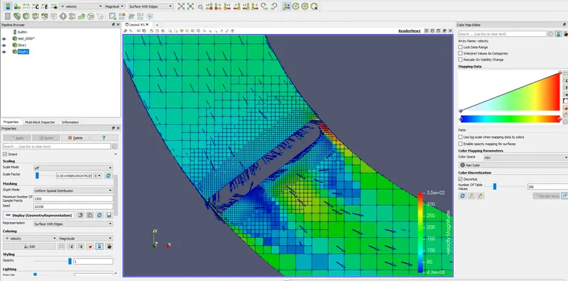
Pressure Contour:
Plotting:
Total Pressure
Avg Velocity:
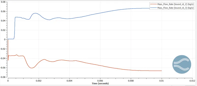
Mass flow rate:
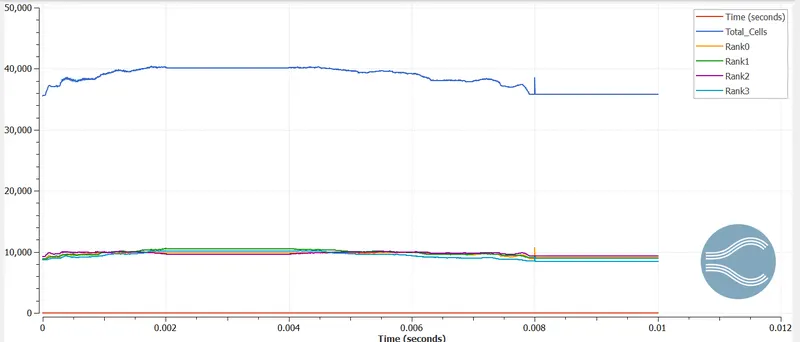
Total cell counts:
Animation of transient flow;
This is the streamlining produced to visualize the flow pattern with static pressure and Throttle at stationary position.
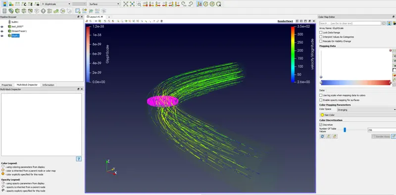
Above is how we simulate the transient flow in ParaView. The animation shows the vector flow and streamlines of the turbulence effect on the fluid. The motion of throttle body has impat on the boundaries making flow a little complex with constant static pressure.