Week 4: Project - Steady state simulation of flow over a throttle body
Aim: Steady-state simulation of flow over a throttle body
Objective:
- To set up and run the steady-state simulation for flow over the throttle body.
- To post-process the results and show pressure and velocity contours.
- To show the mesh (i.e surface with edges)
- To show the plots for pressure, velocity, mass flow rate and total cell count.
- To create an animation in which its throttle movement should be visible.
Introduction
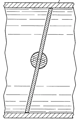
The throttle is a mechanism by which airflow is managed by construction or obstruction in the intake manifold of an SI engine. The throttle valve in the intake system controls the airflow into the engine and thereby cylinder charge, which determines the engine power and torque output. Variation in throttle angle governs the engine speed and torque output by adjusting the airflow into the engine. In a typical SI engine, a throttle valve in the form of circular plate is located in the airflow passage of intake manifold.
Theory:
Throttle
In fuel-injected engines, the throttle body is the part of the air intake system that controls the amount of air flowing into the engine, in response to driver accelerator pedal input in the main. The throttle body is usually located between the air filter box and the intake manifold, and it is usually attached to, or near, the mass airflow sensor. Often, an engine coolant line also runs through it for the engine to draw intake air at a certain temperature and therefore with a known density. The largest piece inside the throttle body is the throttle plate, which is a butterfly valve that regulates the airflow.
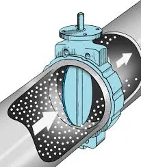
On many cars, the accelerator pedal motion is communicated via the throttle cable, which is mechanically connected to the throttle linkages, which, in turn, rotate the throttle plate. In cars with electronic throttle control (also known as "drive-by-wire"), an electric actuator controls the throttle linkages and the accelerator pedal connects not to the throttle body, but to a sensor, which outputs a signal proportional to the current pedal position and sends it to the ECU. The ECU then determines the throttle opening based on the accelerator pedal's position and inputs from other engine sensors such as the engine coolant temperature sensor. Throttle body showing throttle position sensor. The throttle cable attaches to the curved, black portion on the left. The copper-coloured coil visible next to this returns the throttle to its idle (closed) position when the pedal is released. When the driver presses on the accelerator pedal, the throttle plate rotates within the throttle body, opening the throttle passage to allow more air into the intake manifold, immediately drawn inside by its vacuum. Usually, a mass airflow sensor measures this change and communicates it to the ECU. The ECU then increases the amount of fuel injected by the injectors in order to obtain the required air-fuel ratio.
Steady-State Flow Over the throttle Body
Geometry Setup:
1. Import Geometry:
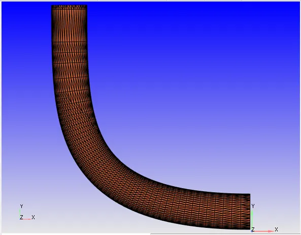
Imported the .stl file geometry.
2. Scaling down the geometry
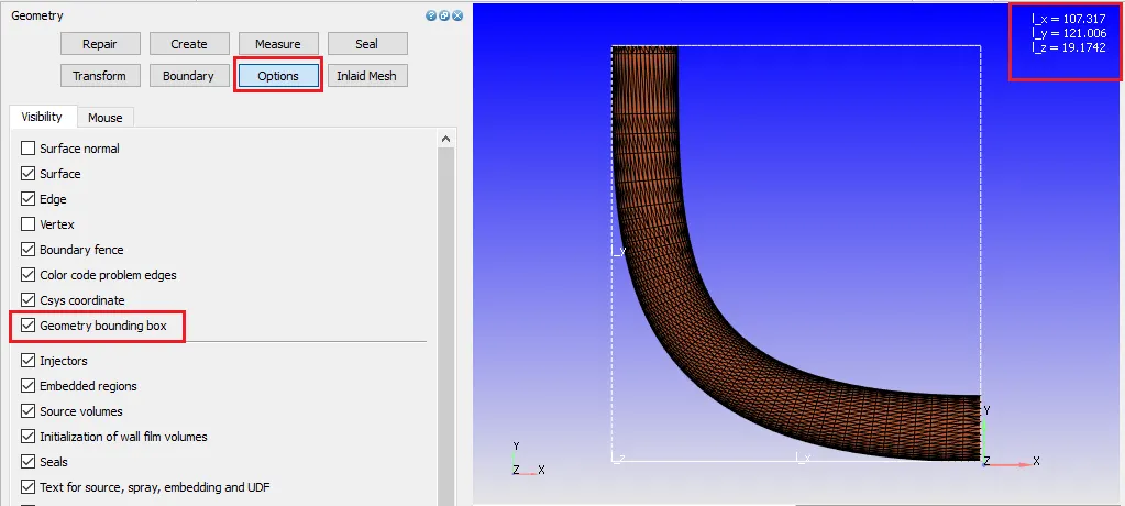
Converge assumes the dimensions in metres i.e in below-shown image l_x=107.317m, l_y=121.006m, l_z=19.1742m which is too large to handle. So, need to scale down.
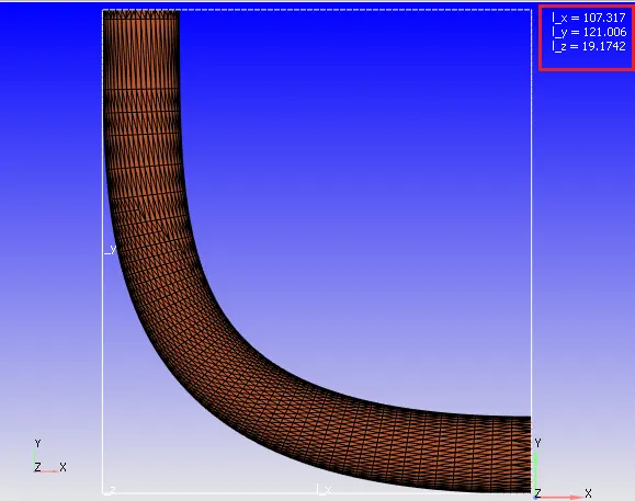
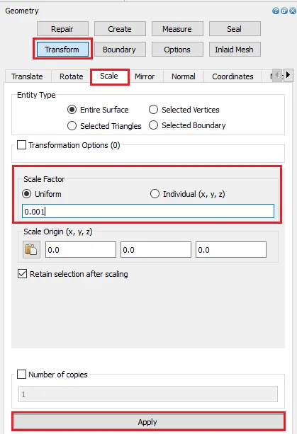
Steps to scale down the geometry:
Geometry>Transform>Scale>Entity Type-Entire Surface>Scale Factor-Uniform=0.001>Apply
Desired Scaled-down Geometry:
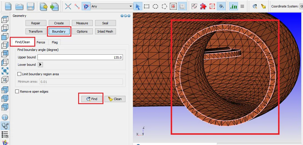
3. Creating a Boundary Fence:
To automatically create a boundary fence-
Geometry>Boundary>Find/Clean>Find
4. Deleting Thickness:
The flow is to be simulated inside the elbow so the thickness of the elbow must be converted to the flow region.
The imported elbow geometry has a particular thickness which is of not much importance.
`therefore` deleting the thickness:
`triangle` as an entity selection-By Angle `20^0`>using cursor pick option>selecting the unwanted thickness>with hot press key enabled>press 'D'
Thickness is deleted.
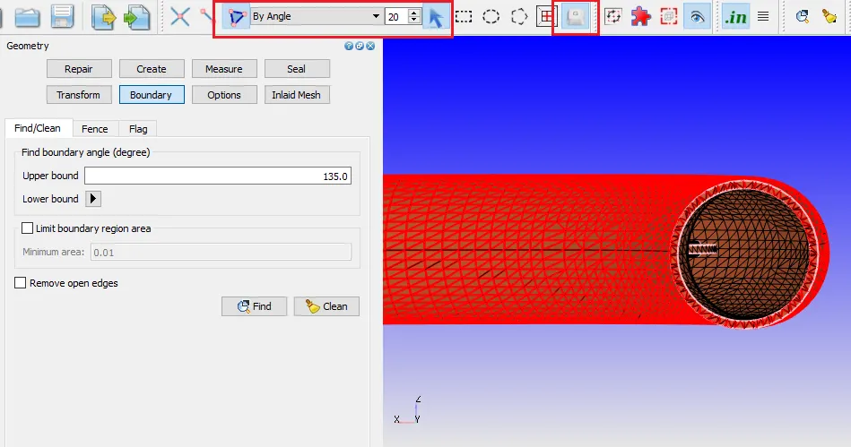
Deleting the thickness of an elbow leads to open edges. Need to close the open edges.
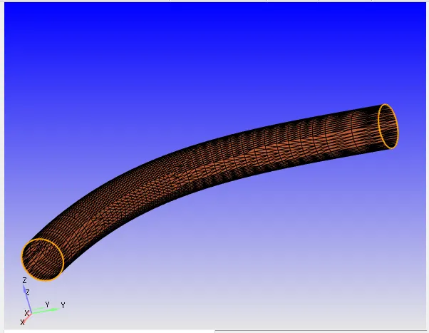
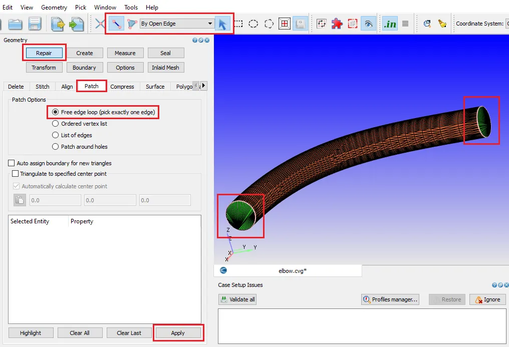
5. Closing open edges
Geometry>Repair>Patch>Patch options-Free Edge Loop>Entity Edge-By Open Edge>Select the edge>Apply and Selecting another open edge>Apply
The elbow edges are closed and that has triangles on its face.
6. Creating Boundaries:
Geometry>Boundary>Flag> '+' create a new boundary>Create Multiple boundaries>OK
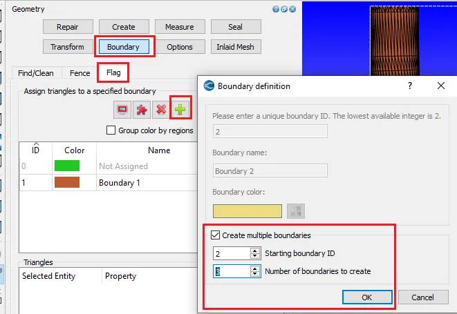
Boundaries are Created:
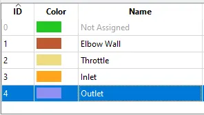
7. Assigning Boundaries:
In converge every part of geometry is assumed to be a triangle. Selecting triangles and grouped so as to assign to specific boundaries.
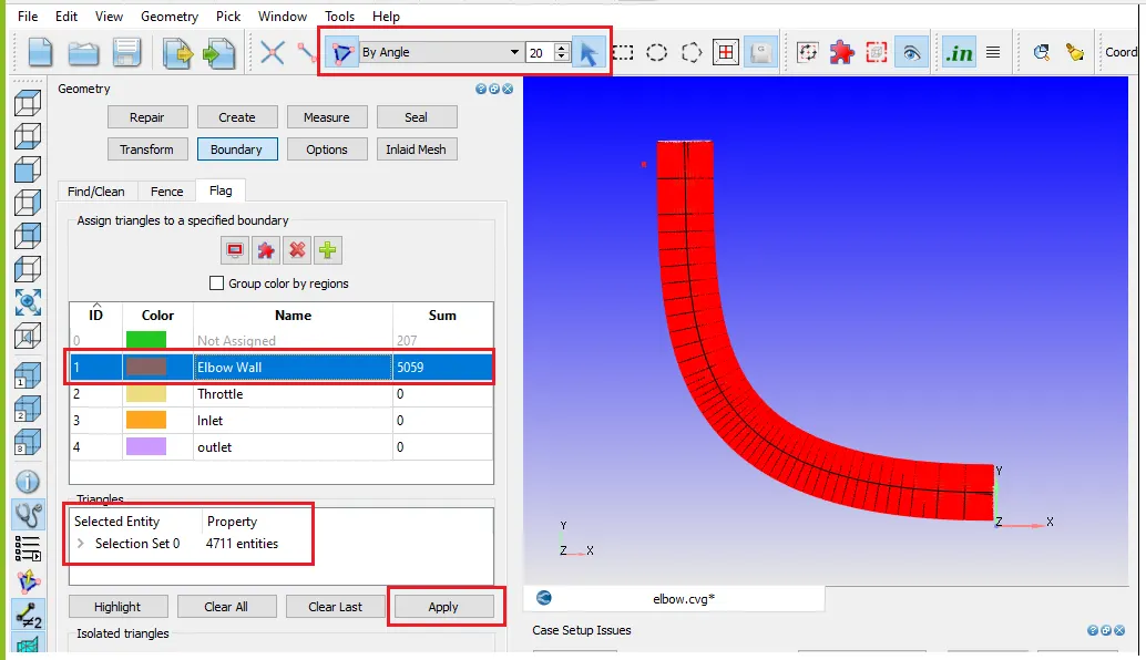
i) Elbow Wall:
`triangle` as an entity selection-By Angle `20^0`>using cursor pick option>Selecting the triangles as shown in below image>Assigning them to Elbow wall Boundary> Apply
ii) Throttle:
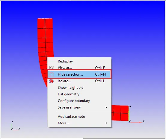
The throttle is located inside the elbow wall, to assign that to a particular boundary- hide the elbow wall.
`triangle` as an entity selection-By Angle `20^0`>using cursor pick option>Selecting the triangles as shown in below image>right click and>Hide selection.
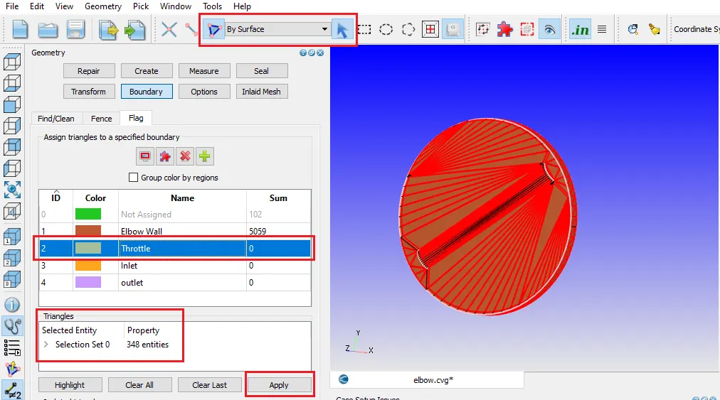
`triangle` as an entity selection-By Surface>using cursor pick option>Selecting the triangles as shown in below image>Assigning them to Throttle Boundary> Apply
Need to select the entire throttle plate because it is not connected to elbow pipe anywhere, it is a separate close surface.
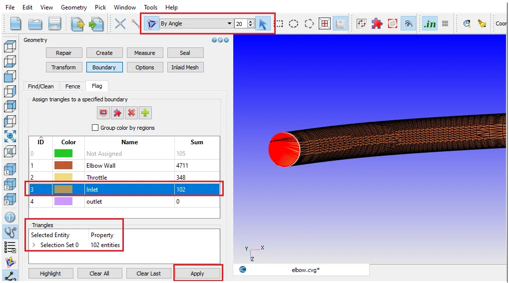
iii) Inlet:
Using right-click and selecting the redisplay option, will display the earlier hidden portion.
`triangle` as an entity selection-By Angle `20^0`>using cursor pick option>Selecting the triangles as shown in below image>Assigning them to Inlet Boundary> Apply
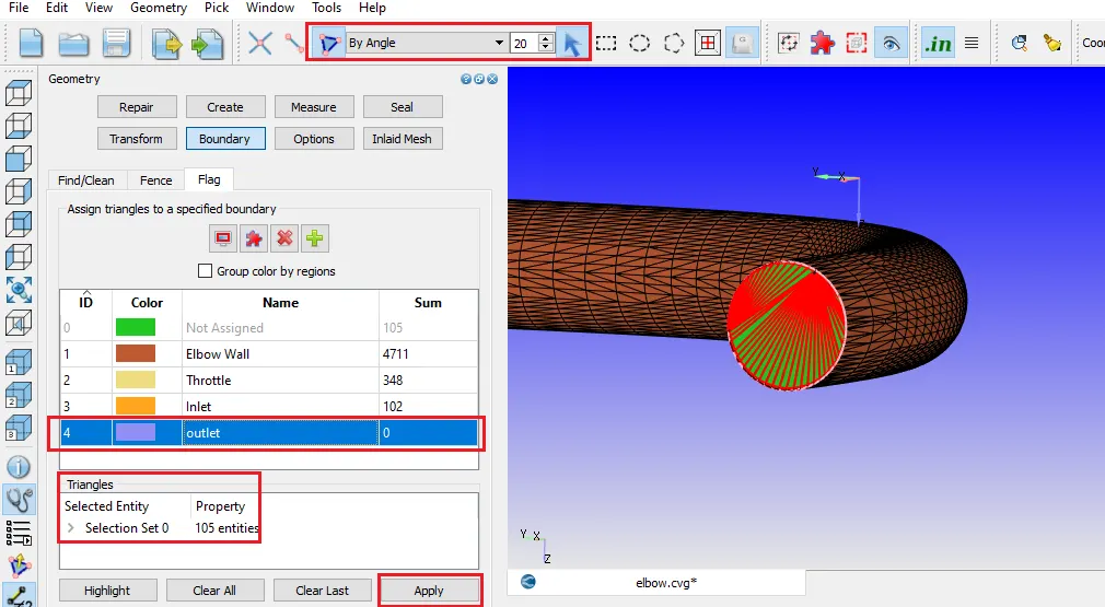
iv) Outlet:
`triangle` as an entity selection-By Angle `20^0`>using cursor pick option>Selecting the triangles as shown in below image>Assigning them to Outlet Boundary> Apply
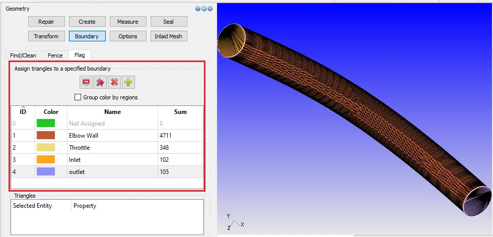
The geometry with assigned boundaries:
8. Normal Orientation:
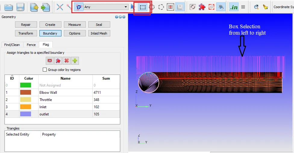
To check the normals first need to hide the half portion of elbow wall.
`triangle` as an entity selection-By Any>using box select option>box selection from left to right shown in below image>triangles will get selected.
On the selected triangles using right-click hiding the selection.
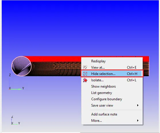
Now with the hidden portion, normal orientation can be viewed.
Every geometry has a normal vector, it basically points perpendicular to it.
Normal Toggle - Enables Normal
In order to run the CFD simulation, the normal should point towards the fluid.
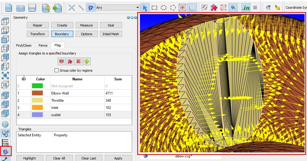
Normals are pointing towards the fluid.
9. Diagnosis:
Run a diagnosis check to ensure that there are no errors. Enable "Check that all the normals are pointing to the interior" then click on find.
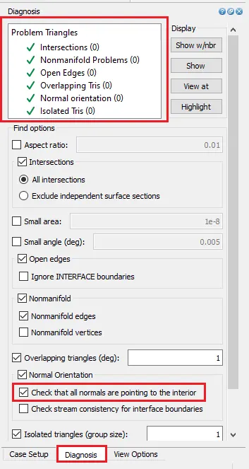
All green ticks under problem triangles show that geometry has no errors.
Case Setup:
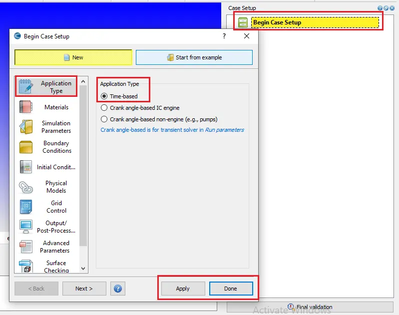
1. Application Type
Application Type - Time-Based
2. Materials
Selecting Air in the drop-down menu of predefined mixtures and keeping Gas Simulation enabled.
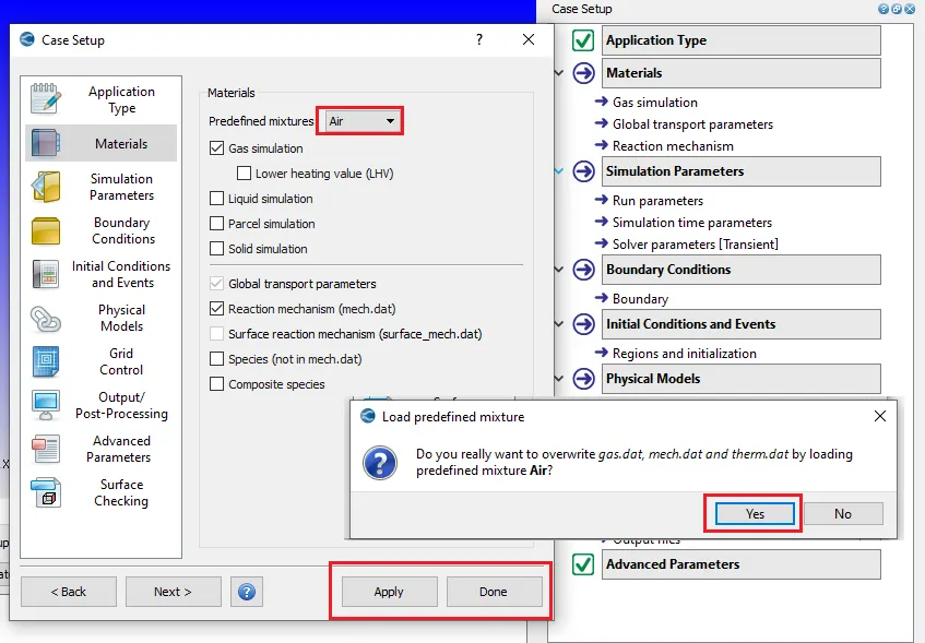
Confirming the permission to overwrite the gas.dat, mech.dat and therm.dat by loading predefined mixture Air.
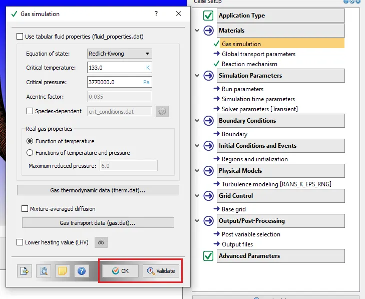
i) Gas Simulation
Keeping the default values for gas simulation > OK
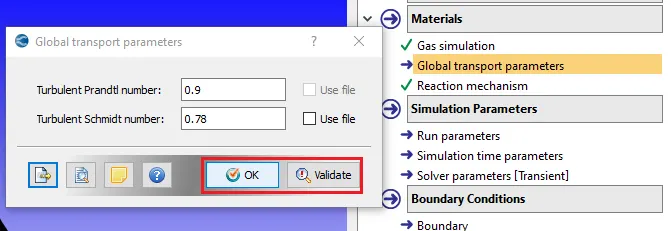
ii) Global Transport Properties
Keeping all the default values for global transport properties > OK
3. Simulation Parameters
i) Run Parameters
Under Solver tab change the solver to Steady-state solver.
Simulation mode is Full hydrodynamic and Gas flow solver is Compressible.
The steady-state solver is used because the valve is not moving.
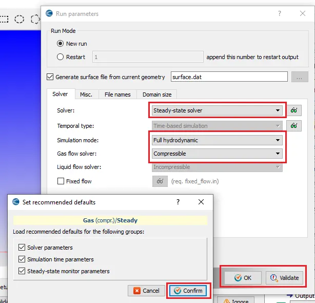
Confirm the recommended defaults permission.
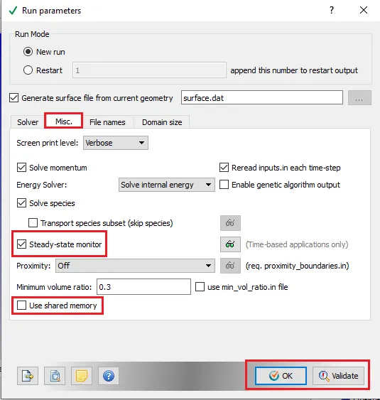
a) Misc. Tab:
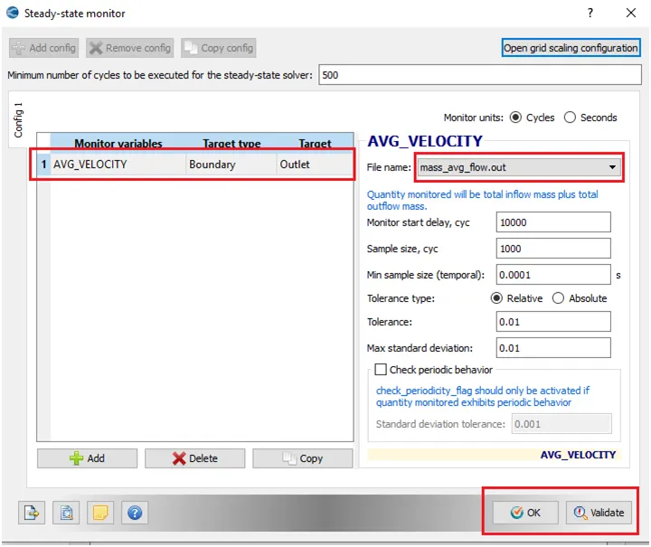
Under Misc. tab checking the Steady-state monitor option and disabling use shared memory option > OK.
b) Steady-state monitor:
ii) Simulation Time Parameters
Set the start time as 0, end time as 15000 cycles, Initial and minimum time step as 1e-6 and Maximum time step as 1 second.
Keep all the other CFL values default > OK.
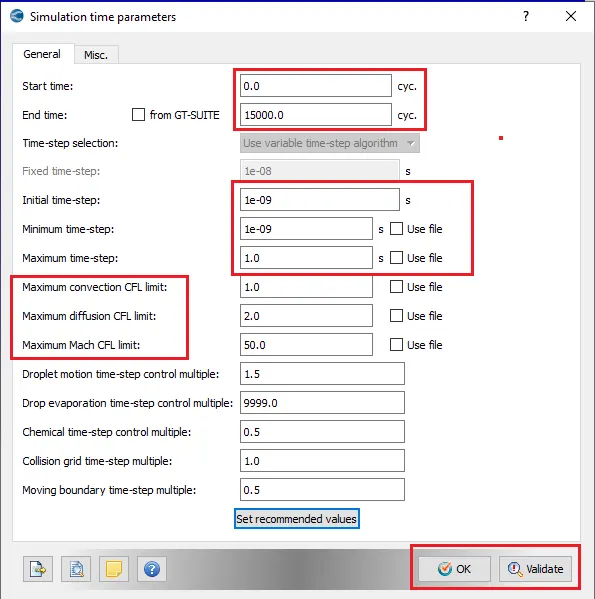
Using initial and maximum time-step as 1e-9 because converge uses a dynamic time-step algorithm. At each and every time-step converge tries to see if the time-step can be increased for next coming time-step.
So, if initial conditions and mesh conditions are good then time is going to increase automatically.
iii) Solver Parameters
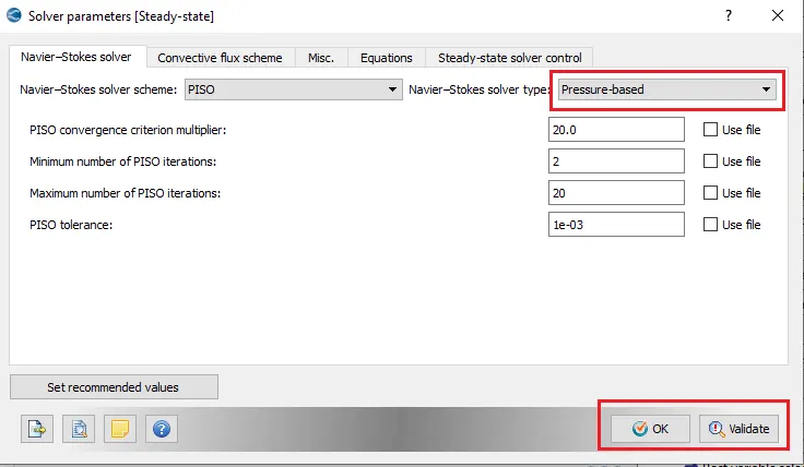
Changing the Navier-stokes solver type as Pressure-based.
Keeping all other settings as default > OK.
4. Regions and Initializations
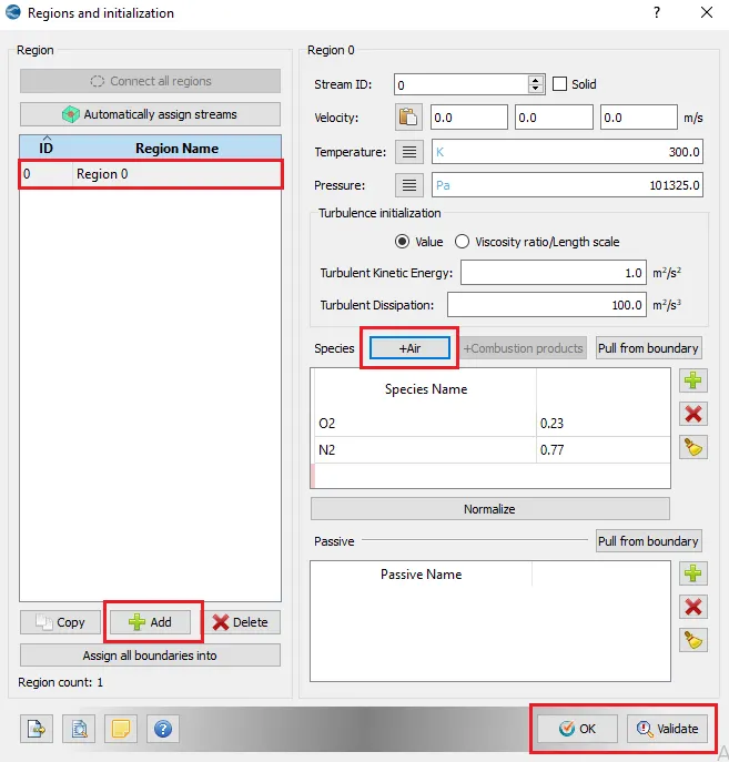
Grouping the boundaries to form volumetric zones called region. This defines a volumetric region with initial conditions like initial pressure, initial temperature, velocity and species concentration
Selecting Add to create a new region, then selecting Air for Species initial conditions and keep the other values default > OK.
5. Boundary
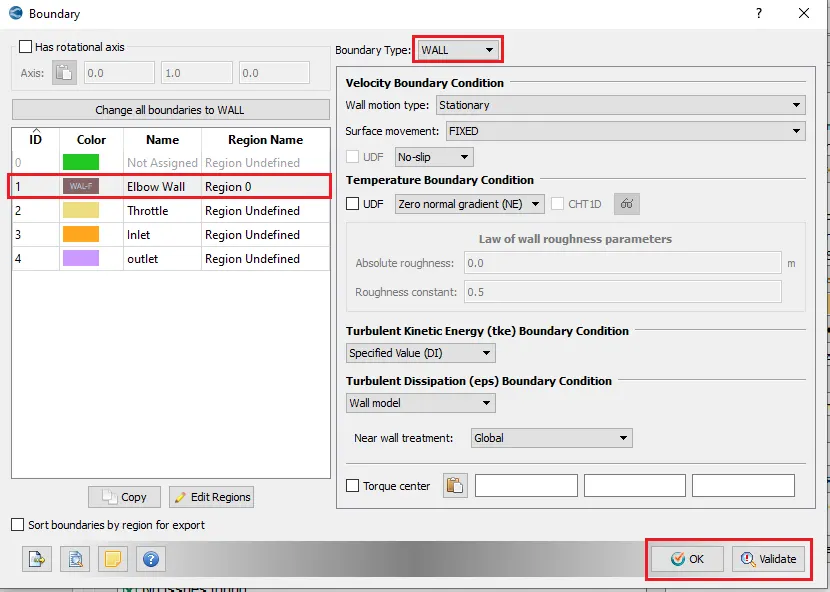
i) Elbow Wall:
Setting boundary type - WALL
Assigning Region0 under region name.
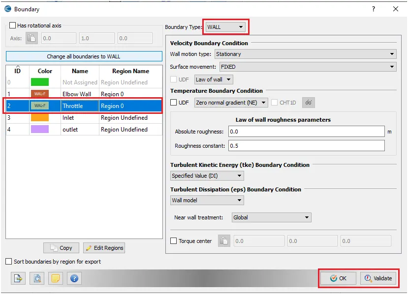
ii) Throttle:
Selecting the boundary type - WALL
Law of the wall is applicable as the flow regime is turbulent.
Assigning Region0 under region name.
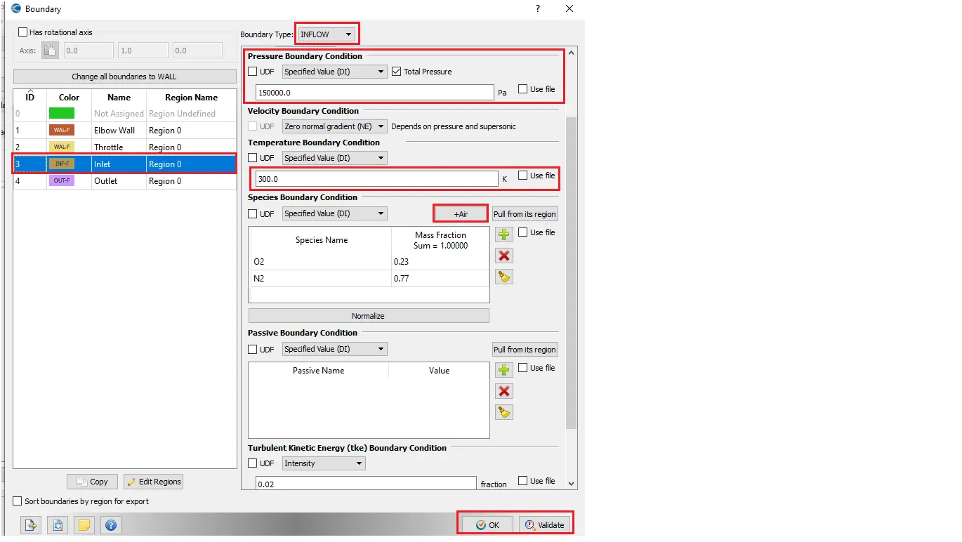
iii) Inlet:
Boundary Type - INFLOW
Pressure boundary condition as the specified value of 1.5e5 Pa i.e 1.5 Bar
keeping the temperature boundary condition as default
Selecting air under the species boundary condition.
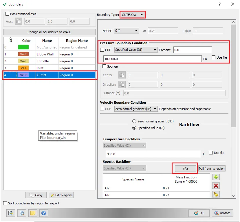
iv) Outlet:
For Outlet set the Pressure Boundary condition as Specified Value of 1e5
Boundary Type - OUTFLOW
Pressure boundary condition as the specified value of 1e5 Pa
Keeping the temperature boundary condition as default
Selecting Air for species backflow
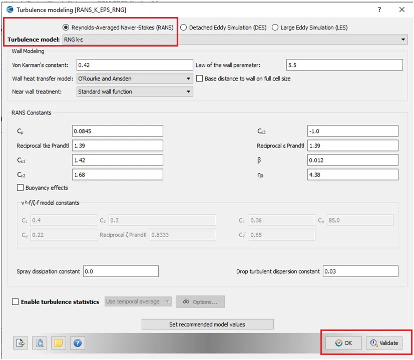
5. Turbulence Modeling:
Keep the Turbulence model as RNG k-epsilon
Keep all the settings default > OK.
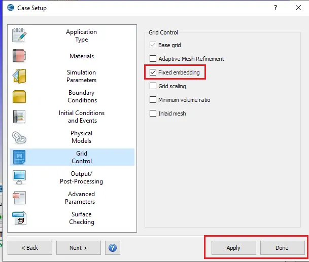
6. Grid Control
Enabling Fixed Embedding option.
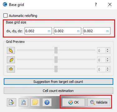
i) Base Grid
Set the mesh size to 2e-3
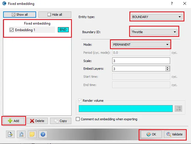
ii) Fixed Embedding
We want finer mesh around the throttle and it can be achieved using Fixed Embedding.
Selecting Add then setting Entity type - BOUNDARY,
Boundary ID - Throttle
Scale - 3 and Embed Layers - 3.
7. Output/Post-Processing
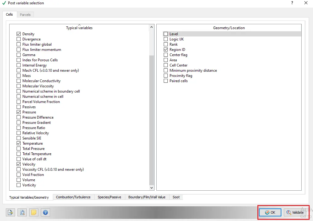
i) Post-Variable Selection
Using default settings
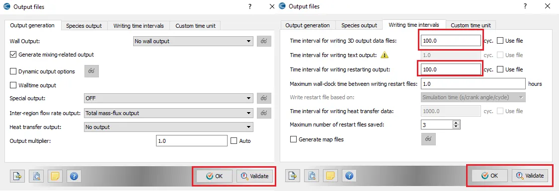
ii) Output Files
Setting the time interval for writing 3D output data files and interval for writing restarting output to 100 and keep all the other values default > OK
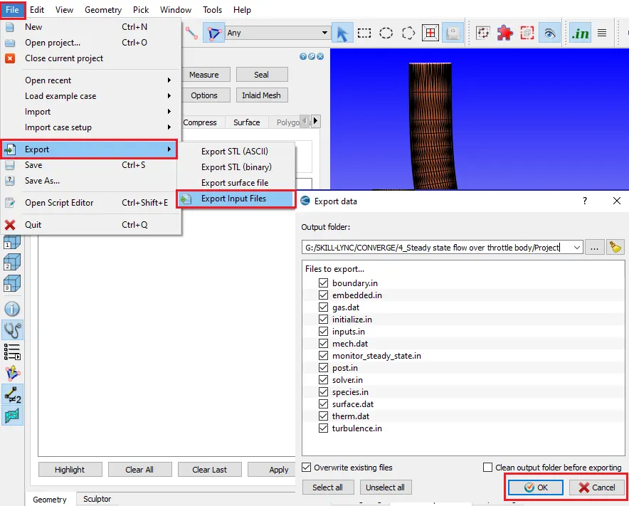
8. Export all the input files
Export all the input files into a separate folder
Files>Export>Export Input Files>setting up the desired location>OK
9. Copy and paste the mpiexec.exe file to the input files folder
Run Simulation
Cygwin - Cygwin is a collection of GNU and open-source tools that provide functionality similar to Linux distribution on windows.
To run the simulation, open Cygwin and navigate to the folder in which the input files are exported.
To run the simulation command with executable to be entered
$ mpiexec.exe -n 2 converge-intelmpi.exe restricted </dev/null> logfile.txt &
Taking output mpiexec.exe and sending it to </dev/null> further Taking data from </dev/null> and sending to logfile.txt
Post convert all the output files
Enter the case name, select the file type as EnSight format, select boundary surface output to yes, navigate to the directory where the output files are located.
Then for files select all, for cell variables select all and hit Convert. The file will be with case name in .case format
Post-processing
Launch Paraview from ...ParaView-5.4.1-Qt5-OpenGL2-Windows-64bitbin folder and open the .case file and press apply.
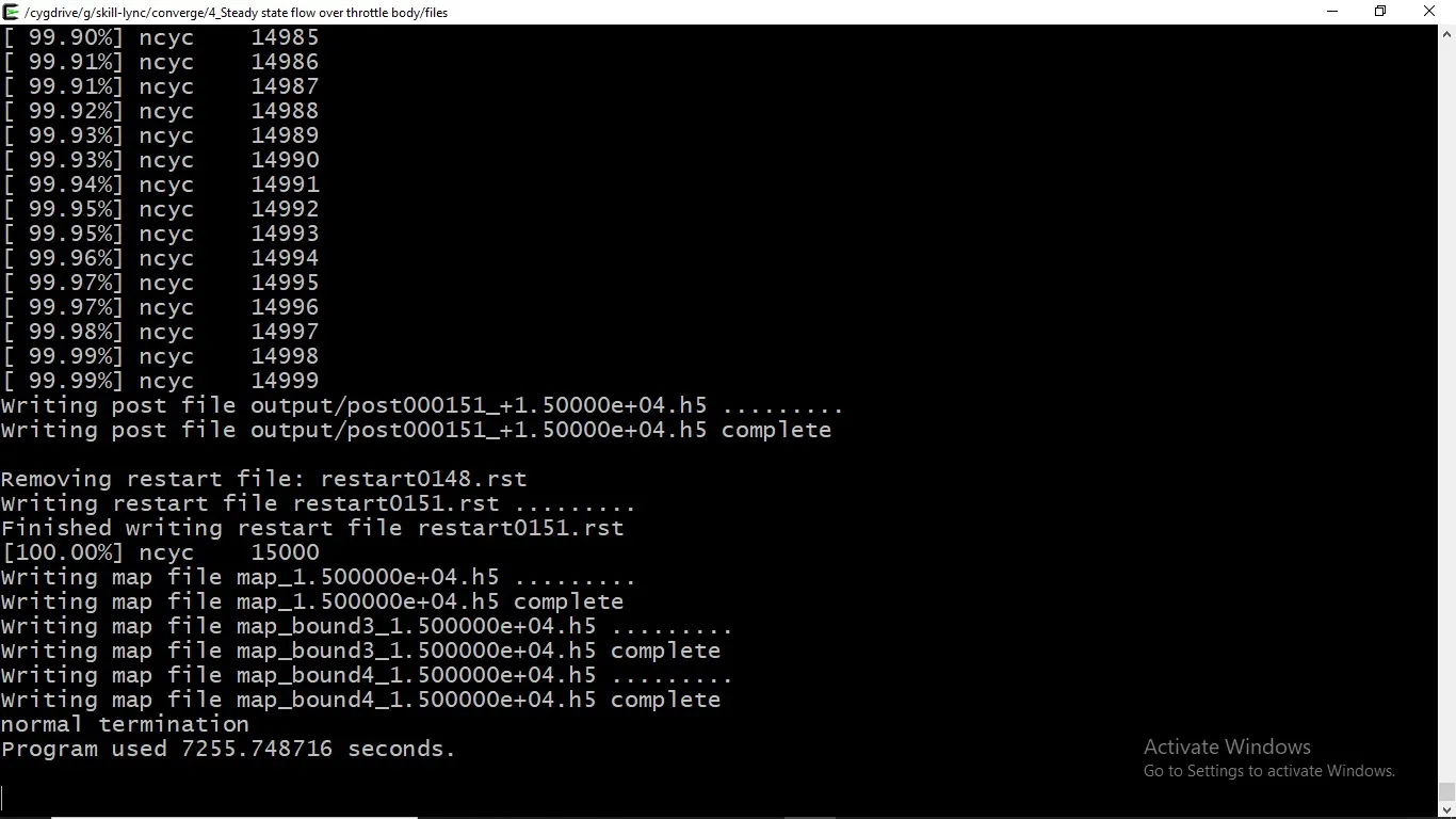
Computational Time:
Simulation Results:
Mesh
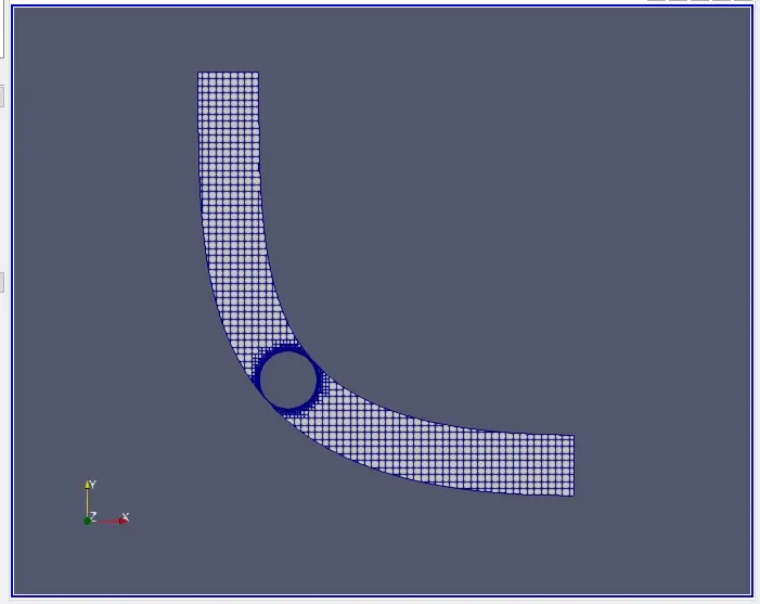
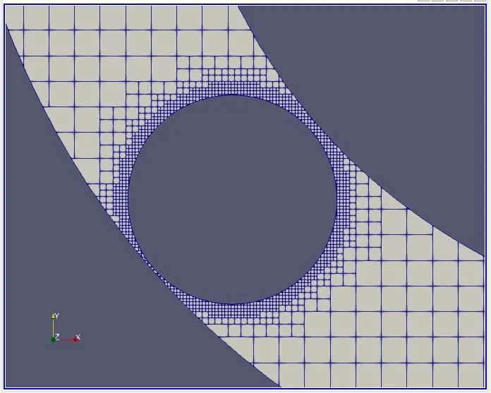
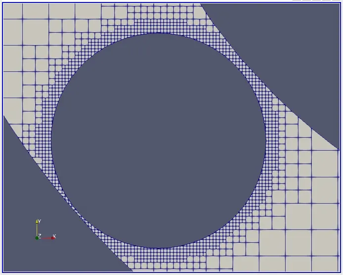
The 'fixed embedding' created a fine mesh near the 'Throttle body'. The scale parameter (n) determines the final size of elements as `dx/(2^n)` and layers determines the number of layers of fine mesh along the boundary. The software creates the gradual fine mesh by dividing neighbouring cells of boundary into half the size of the previous cell, till the finest size becomes as decided by the scale parameter.
Pressure and Velocity Contours
Pressure Contour
 .
.
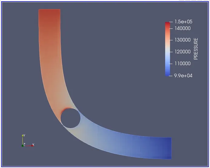
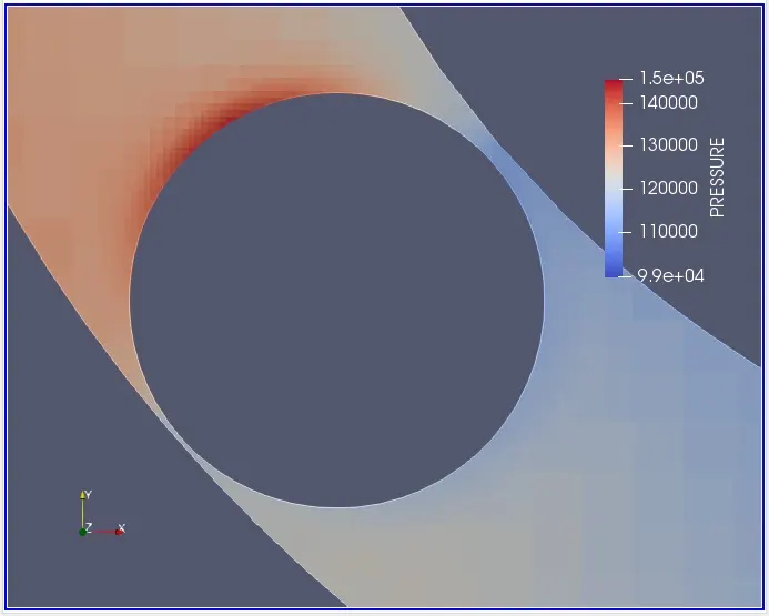
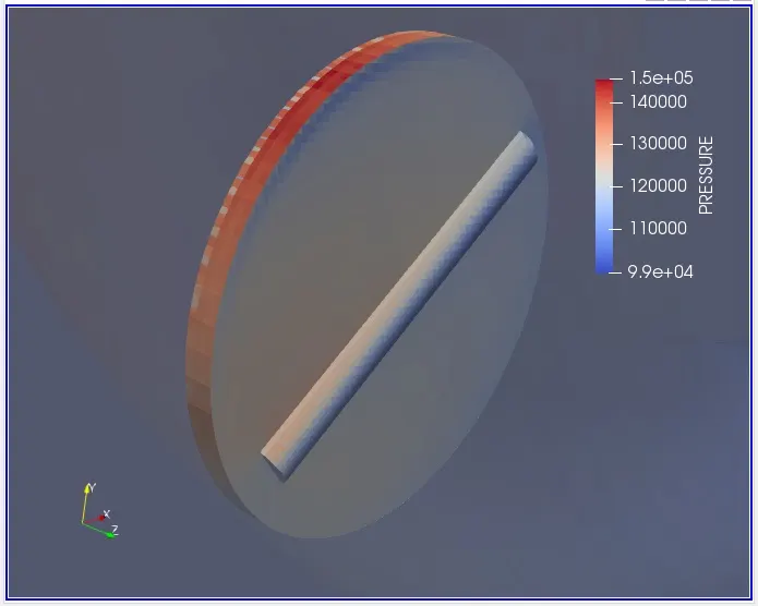
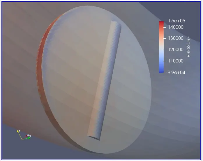
The throttle face which is facing towards the flow is more intensive as the fluid interacts with the throttle and the velocity decreases along the surface thus this face has more pressure than the other face of throttle where the fluid has no resistance. The total and static pressure at each side is reasonable as the static pressure decreases along the flow and total pressure increases along the flow. The total pressure is the sum of static and dynamic pressure the dynamic pressure is a function of velocity since the velocity of the flow increases so the total pressure increases.
Throat region has the minimum area available for the air to flow. In order to reduce energy loss, the flow gets accelerated at the throat. Hence, the pressure drop at the throat is minimum due to the maximum velocity.
The static pressure at the start drops due to the increase in velocity, as per conservation law and then gets stable as the simulation proceed
Pressure Animation:
Pressure Plot:
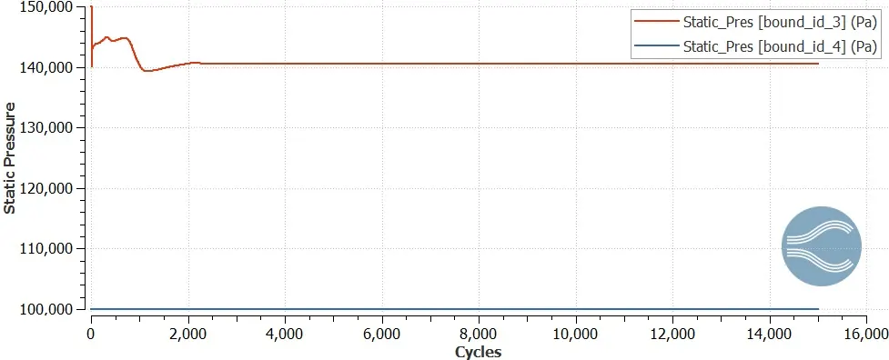
The static pressure at the start drops due to the increase in velocity, as per conservation law and then gets stable as the simulation proceeds.
Velocity Contour Plot
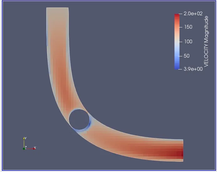
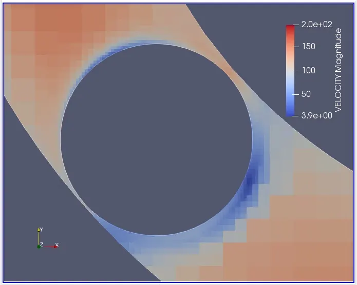
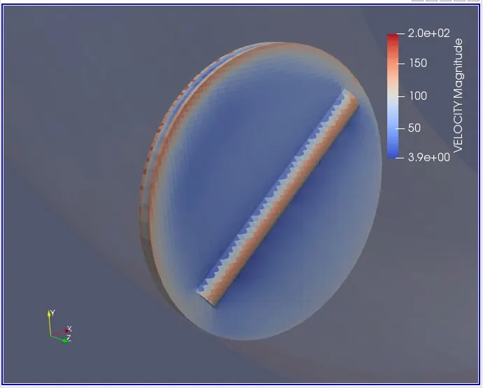
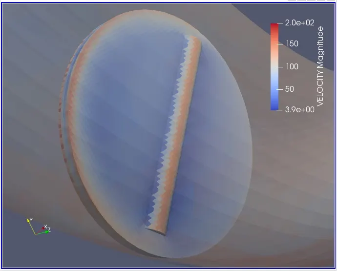
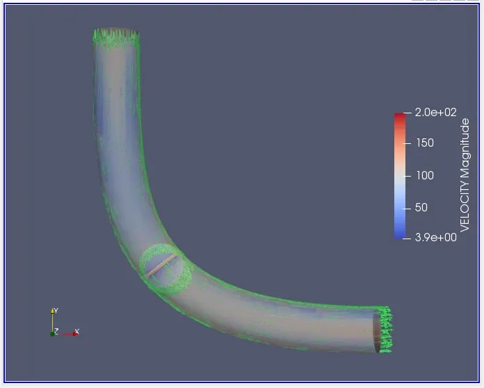
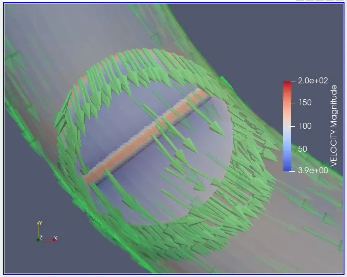
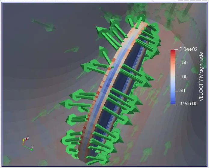
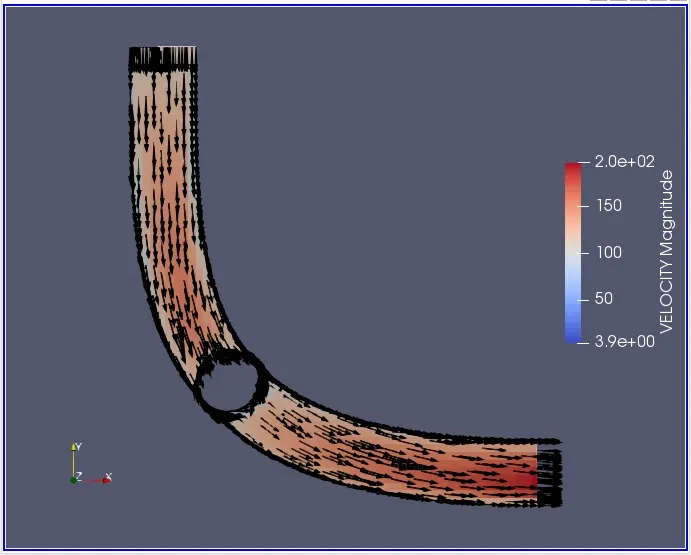
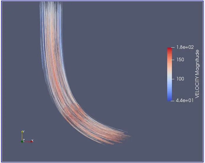
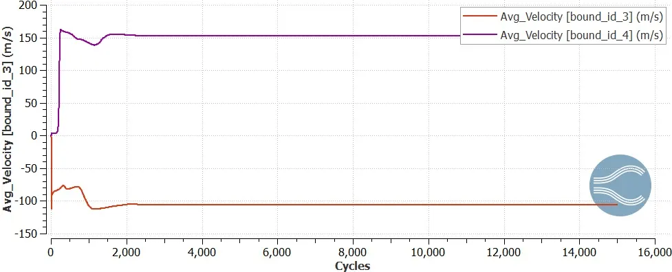
The geometry of the throttle is placed in such that a small gap between throttle and wall which is not in the actual case, so the velocity at the throttle end is not the actual value. The dip in the velocity curve which is due to the interaction with the throttle and as the flow progresses the velocity becomes steady. The decrease of pressure in the throttle which causes cavity which increases the velocity of the flow.
The throttle plate and the throttle shaft provide restriction to the flow of intake air. Lesser is the restriction across the flow, lower is the loss of energy. This increases the velocity at the outlet of the throttle body.
Velocity Vector Propagation:
Velocity Streamlines:
Velocity Animation:
Velocity Plot:
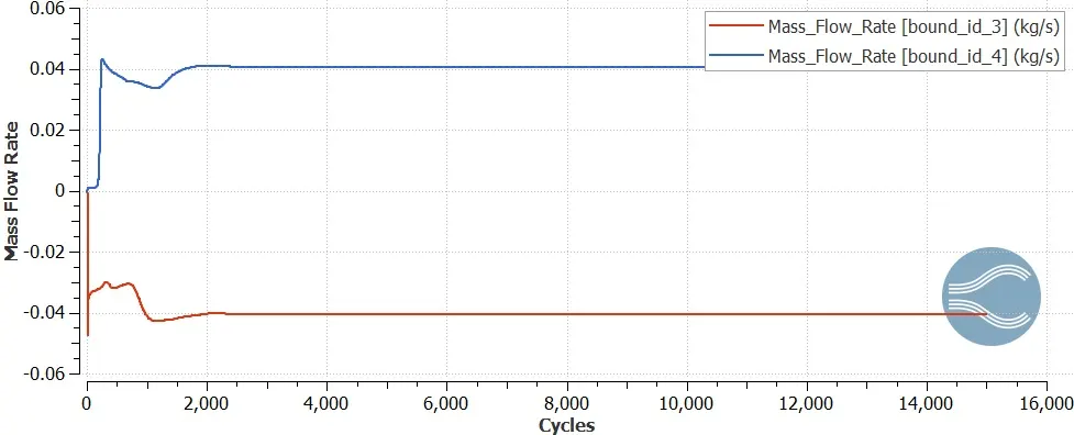
Mass Flow Rate Plot:
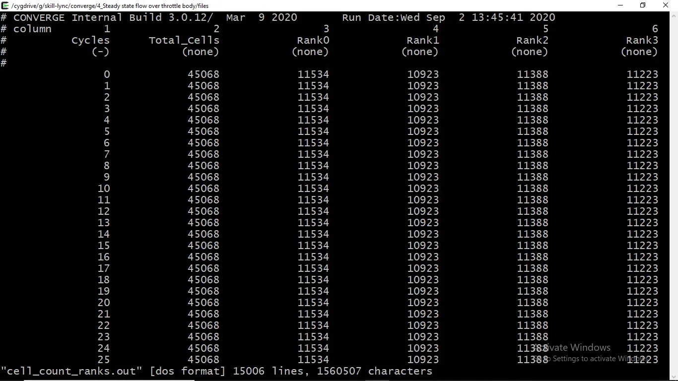
Total Cell Count Plot
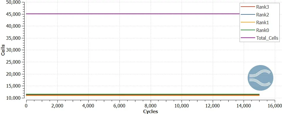
Cell Count:
Conclusions:
1. The mass flow rate initially takes a little turbulence and finally converges as expected. It can be clearly seen from the graph that the law of conservation of the mass is followed as the inflow mass flow rate is balanced by the outflow mass flow rate.
2. The throttle plate and the throttle shaft provide restriction to the flow of intake air. Lesser is the restriction across the flow, lower is the loss of energy. This increases the velocity at the outlet of the throttle body.
3. Throat region has the minimum area available for the air to flow. In order to reduce energy loss, the flow gets accelerated at the throat. Hence, the pressure drop at
the throat is minimum due to the maximum velocity.
4. The static pressure at the start drops due to the increase in velocity, as per conservation law and then gets stable as the simulation proceeds.