Week 4 - Genetic Algorithm

AIM:

To devolop a code in Matlab to optimize the stalagmite function and find the global maxima of the function.

INTRODUCTION:

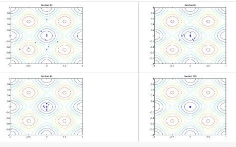
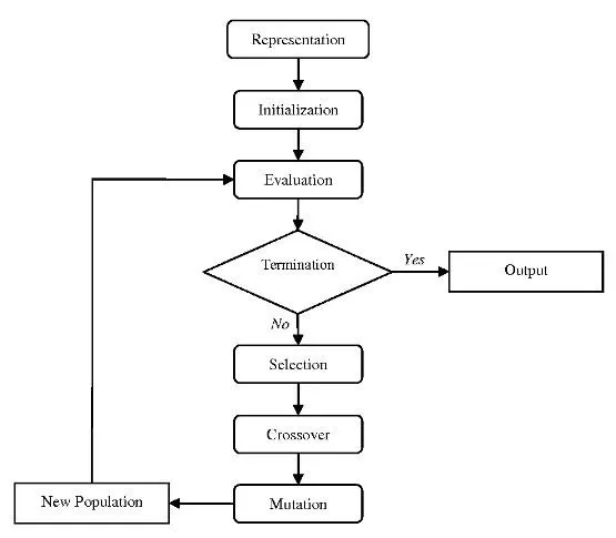
The genetic algorithm is inspired by the process that drives biological evolution. The process of evolution starts with the selection of fittest individuals from a population. Then they produce offspring which inherit the characteristics of the parents and will be added to the next generation. If parents have better fitness, their offspring will be better than parents and have a better chance at surviving. This process keeps on iterating and at the end, a generation with the fittest individuals will be found. And this is the main working principle for the algorithm because at each step, the genetic algorithm selects randomly from the current population to be parents and uses them to produce the children for the next generation.

Over successive generations, the population evolves toward an optimal solution. The genetic algorithm can be applied to solve a variety of optimization problems that are not well suited for standard optimization algorithms, including problems in which the objective function is discontinuous, nondifferentiable, stochastic, or highly nonlinear.

The genetic algorithm uses three main types of rules at each step to create the next generation from the current population:

• Selection rulesselect the individuals, called parents, that contribute to the population at the next generation.
• Crossover rulescombine two parents to form children for the next generation.
• Mutation rulesapply random changes to individual parents to form children.

A) Selection

The idea of the selection phase is to select the fittest individuals and let them pass their genes to the next generation. The main goal of this phase is to find the region where the chances of getting the best solution are more.

GA tries to move the genotype to higher fitness in the search space.Too strong fitness selection bias can lead to sub-optimal solutions.Too little fitness bias selection results in unfocused search.

Reproduction

Generation of offspring happen in 2 ways:

• Crossover
• Mutation

B) Crossover

Crossover is the most significant stage in the genetic algorithm. During crossover, a random point is selected while mating a pair of parents to generate offspring.

There are 3 major types of crossover.

 Single Point Crossover: A point on both parents’ chromosomes is picked randomly, and designated a ‘crossover point’.

Two-Point Crossover: Two crossover points are picked randomly from the parent chromosomes.

Uniform Crossover: In a uniform crossover, typically, each bit is chosen from either parent with equal probability. The new offspring are added to the population.

C) Mutation

In a few new offspring formed, some of their genes can be subjected to a mutation with a low random probability. This indicates that some of the bits in the bit chromosome can be flipped. Mutation happens to take care of diversity among the population and stop premature convergence.

MATLAB CODE:

(i) Stalagmite function code for calling in the main code:

function [f] = stalagmite(input_vector);
x = input_vector(1);
y = input_vector(2);
f1x = (sin((5.1*pi*x)+0.5))^6;
f1y = (sin((5.1*pi*y)+0.5))^6;
f2x = exp(-4.*log(2)*(((x-0.0667)^2)/(0.64)));
f2y = exp(-4.*log(2)*(((y-0.0667)^2)/(0.64)));

f = -(f1x.*f1y.*f2x.*f2y);  
end

 1. A function f is called with the input variable called input_vector.

2. Next the X and Y values are assigned separetely.

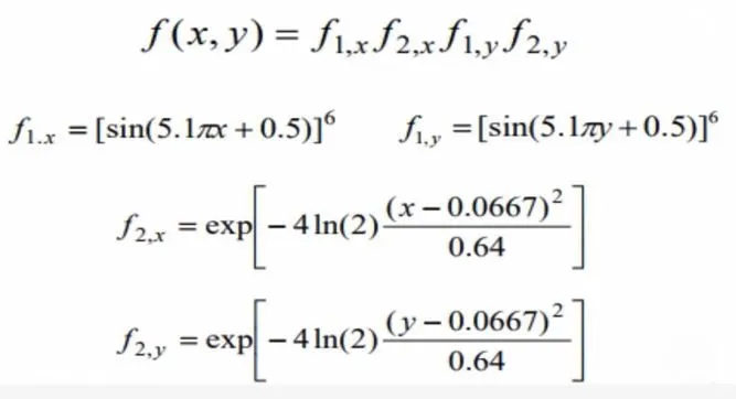
3. Inorder to plot the graph in the main code, following below formulas are used to define the fittness function.

(ii) Main code:

clear all
close all
clc

% Creating 1D array with defining x and y values range
x = linspace(0,0.6,150);  
y = linspace(0,0.6,150);

%Creating 2D array
[xx yy] = meshgrid(x,y); 
%number of cases
num_cases = 50;

%Function for surface plot
for i=1:length(xx)
    for j=1:length(yy)
        input_vector(1) = xx(i,j);
        input_vector(2) = yy(i,j);
        f(i,j) = stalagmite(input_vector); % Function calling
    end
end

% Function to calculate the coordinate points of ,y,function values at each
% point- Unbounded condition
tic
for i=1:num_cases
    [inputs1,fopt1(i)] = ga(@stalagmite,2); % ga function
    xopt(i) = inputs1(1);
    yopt(i) = inputs1(2);
    
end

% Graph for surface plot and Foptimum
study1_time = toc;
figure(1)
subplot(2,1,1)    % Subplot(m,n,p)
surfc(x,y,-f)     % Surface plot
shading interp;   % To get smooth surface
xlabel('X axis')  % Labelling
ylabel('Y axis')
zlabel('Function value')
hold on
plot3(xopt,yopt,-fopt1,'marker','o','markersize',5,'markerfacecolor','r') % plot co-ordinates
title('Unbounded statistical behaviour')
subplot(2,1,2)
plot(-fopt1)      % Graph for Foptimum
xlabel('Iterations')
ylabel('function value')

% Statistical condition with upper and lower bounds(0->0.5):

tic
for i=1:num_cases
    [inputs2,fopt2(i)] = ga(@stalagmite,2,[],[],[],[],[0;0],[0.5;0.5]); % ga syntax with upper and lower bound
    xopt(i) = inputs2(1);
    yopt(i) = inputs2(2);
    
end

% Graph plot
study2_time = toc;
figure(2);
subplot(2,1,1)
surfc(x,y,-f)
shading interp;
xlabel('X axis')
ylabel('Y axis')
zlabel('Function value')
hold on
plot3(xopt,yopt,-fopt2,'marker','o','markersize',5,'markerfacecolor','r')
title('Bounded statistical behaviour')
subplot(2,1,2)
plot(-fopt2)
xlabel('Iterations')
ylabel('function value')

% Boundeed statistical cond. with increase in population:
%options = optimoptions('ga')
options = optimoptions('ga','populationsize',170); % Changing the default values

% Function for the above case
tic
for i=1:num_cases
    [inputs3,fopt3(i)] = ga(@stalagmite,2,[],[],[],[],[0;0],[0.5;0.5],[],[],options);
    xopt(i) = inputs3(1);
    yopt(i) = inputs3(2);
    
end
study3_time = toc;

% Graph plot
figure(3);
subplot(2,1,1)
surfc(x,y,-f)
shading interp;
xlabel('X axis')
ylabel('Y axis')
zlabel('Function value')
hold on
plot3(xopt,yopt,-fopt3,'marker','o','markersize',5,'markerfacecolor','r')
title('Bounded statistical behaviour with increase in population')
subplot(2,1,2)
plot(-fopt3)
xlabel('Iterations')
ylabel('function value')

% Print the values of x and y coordinates of global maxima and Foptimum:
% Calculating the time taken for each case 

fprintf (' The Results of each cases are Below :\n')
fprintf (' Study 1 : Unbounded Statistical Behvaiour \n')
fprintf (' The Time taken for the study 1 is : %f \n',study1_time)
fprintf (' The Co-ordinates of x and y for the Global Maxima of the Function are : %f,%f \n',inputs1(1),inputs1(2))
fprintf (' The Global Maxima of the Function is : %f \n',-(mean(fopt1)))

fprintf (' Study 2 : Bounded Statistical Behvaiour \n')
fprintf (' The Time taken for the study 2 is : %f \n',study2_time)
fprintf (' The Co-ordinates of x and y for the Global Maxima of the Function are : %f,%f \n',inputs2(1),inputs2(2))
fprintf (' The Global Maxima of the Function is : %f \n',-(mean(fopt2)))

fprintf (' Study 3 : Bounded Statistical Behvaiour with Increased Population Size \n')
fprintf (' The Time taken for the study 3 is : %f \n',study3_time)
fprintf (' The Co-ordinates of x and y for the Global Maxima of the Function are : %f,%f \n',inputs3(1),inputs3(2))
fprintf (' The Global Maxima of the Function is : %f \n',-(mean(fopt3)))

1. x = linspace(0,0.6,150);
    y = linspace(0,0.6,150);

    [xx yy] = meshgrid(x,y);

    num_cases = 50;

    The x and y values are given a value from 0->0.6 with an intervel of 150 values in between them using the function linspace.

2. Now a 2D array is created with all the x and y values in one matrix using the function meshgrid. The number of cases or the total iteration is taken as 50.

3. for i=1:length(xx)
        for j=1:length(yy)
        input_vector(1) = xx(i,j);
        input_vector(2) = yy(i,j);
        f(i,j) = stalagmite(input_vector);
        end
    end

   Inorder to create the surface plot for stalagmite function, the following .The additional created stalagmite function is called in this step.

4. Unbounded Statistical condition:

    tic

    for i=1:num_cases
    [inputs1,fopt1(i)] = ga(@stalagmite,2);
    xopt(i) = inputs1(1);
    yopt(i) = inputs1(2);

    end
    study1_time = toc;

   tic and toc are given inorder to find the total elapsed time for running the loop in between it. Inorder to calculate the value of fitness function at each point of the mesh grid as well as the x and y values at each point,  for loop is used for calculating the x and y values from the above 2D matrix.

5. figure(1)
    subplot(2,1,1)
    surfc(x,y,-f)
    shading interp;
    xlabel('X axis')
    ylabel('Y axis')
    zlabel('Function value')
    hold on
    plot3(xopt,yopt,-fopt1,'marker','o','markersize',5,'markerfacecolor','r')
    title('Unbounded statistical behaviour')
    subplot(2,1,2)
    plot(-fopt1)
    xlabel('Iterations')
    ylabel('function value')

    surfc function is used for surface plotting with x,y and fvalues. f is given negetive as the stalagmite function gives the minimum value in the plot. Inorder to get the global maximum, reverse the f value.

    Shading interp is used to get a smooth surface.

    The subplot(m,n,p) helps to define the grid needed for plotting with the position of each graph. It will create a m*n grid in the plot with deciding the position of each plot to be placed

   

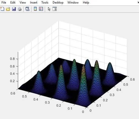
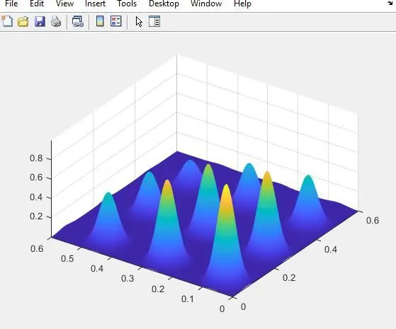
    plot3 function is used to plot the coordinates of the optimum values of x_opt,y_opt and f_optimum

    plot(-fopt1) helps to plot the graph of fopt or the function values vs iterations.

6. Bounded Statistical condition:

    tic
    for i=1:num_cases
    [inputs2,fopt2(i)] = ga(@stalagmite,2,[],[],[],[],[0;0],[0.5;0.5]);
    xopt(i) = inputs2(1);
    yopt(i) = inputs2(2);

    end
    study2_time = toc;

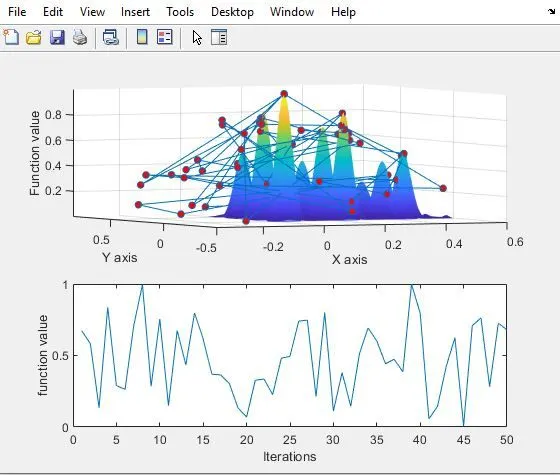
    Now the same function has to be given by defining upper and lower bound to reduce the search area within the range. The range can be inputted with an another syntax of ga.The range is given in between 0->0.5. Since no linear and            non-linear equalities and inequalities exist, it can be given inside empty square brackets.

7. figure(2);
    subplot(2,1,1)
    surfc(x,y,-f)
    shading interp;
    xlabel('X axis')
    ylabel('Y axis')
    zlabel('Function value')
    hold on
    plot3(xopt,yopt,-fopt2,'marker','o','markersize',5,'markerfacecolor','r')
    title('Bounded statistical behaviour')
    subplot(2,1,2)
    plot(-fopt2)
    xlabel('Iterations')
    ylabel('function value')

   As the same done above, the surface plot has to be plotted with shading interp with all three axis to be labelled and title has also to be given. plot3 commands helps to plot the coordinates with hold on has to given to get all graphs and           plots in one figure.

8. Bounded Statistical condition with increase in population size:

    options = optimoptions('ga','populationsize',170);

    tic
    for i=1:num_cases
    [inputs3,fopt3(i)] = ga(@stalagmite,2,[],[],[],[],[0;0],[0.5;0.5],[],[],options);
    xopt(i) = inputs3(1);
    yopt(i) = inputs3(2);

    end

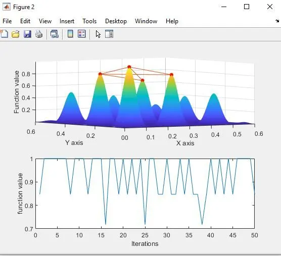
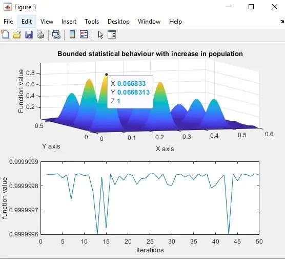
    By increasing the population size of the function, the accuracy of the ga can be increased, which results to give a single point value for every iterations.

    Options are additional features in the matlab which helps to change the default values in the program function. Here, the population size has been changed to 170 from the default value using an inbuilt function called optimoptions.

    A for loop is initiated similar to that of bounded condition but the only difference is in the ga function used.The syntax for ga function used here is shown above

    The coordinates x and y of the global maxima are stored in xopt(i) and yopt(i)

9.  study3_time = toc;
     figure(3);
     subplot(2,1,1)
     surfc(x,y,-f)
     shading interp;
     xlabel('X axis')
     ylabel('Y axis')
     zlabel('Function value')
     hold on
     plot3(xopt,yopt,-fopt3,'marker','o','markersize',5,'markerfacecolor','r')
     title('Bounded statistical behaviour with increase in population')
     subplot(2,1,2)
     plot(-fopt3)
     xlabel('Iterations')
     ylabel('function value')

    A figure 3 graph is plotted for this case. IN figure3 two subplots are plotted.The rest of the functions are similar to what done in the second case.

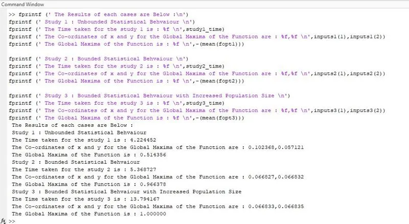
10. At last, fprintf function is used to print the values of coordination and function values in the command window.

GRAPH AND SURFACE PLOTS:

(I) Unbounded Statistical condition:

(II)Bounded Statistical condition:

(III) Bounded Statistical condition with increase in population size:

ERRORS OCCURED:

The normal syntax errors with error in case sensitive characters and paranthesis errors are encountered during the time of coding.

CONCLUSION:

• Learned about new syntax and function like stalagmatic,ga,optimoptions which can be effectivily used for many other coding purposes.
• Usage of increased population method helps to achieve single constant value for all the iterations. The value of fopt remains 1 for all the iterations.