Week 4 - Genetic Algorithm

• Selection rules select the individuals, called parents, that contribute to the population at the next generation.

• Crossover rules combine two parents to form children for the next generation.

• Mutation rules apply random changes to individual parents to form children.

In each generation,the fitness of every indivudual in the population is evaluated.Multiple individuals are selected from the current population and modified to form a new population.

• Start with a large “population” of randomly generated
“attempted solutions” to a problem
• Repeatedly do the following:
– Evaluate each of the attempted solutions
– (probabilistically) keep a subset of the best
solutions
– Use these solutions to generate a new population
• Quit when you have a satisfactory solution (or you
run out of time)

SYNTAX FOR GA:

• x = ga(fun,nvars)
• x = ga(fun,nvars,A,b)
• x = ga(fun,nvars,A,b,Aeq,beq)
• x = ga(fun,nvars,A,b,Aeq,beq,lb,ub)
• x = ga(fun,nvars,A,b,Aeq,beq,lb,ub,nonlcon)
• x = ga(fun,nvars,A,b,Aeq,beq,lb,ub,nonlcon,options)
• x = ga(fun,nvars,A,b,[],[],lb,ub,nonlcon,IntCon)
• x = ga(fun,nvars,A,b,[],[],lb,ub,nonlcon,IntCon,options)
• x = ga(problem)
• [x,fval] = ga(___)
• [x,fval,exitflag,output] = ga(___)
• [x,fval,exitflag,output,population,scores] = ga(___)

SYNTAX DESCRIPTION:

• x = ga(fun,nvars) finds a local unconstrained minimum, x, to the objective function, fun. nvars is the dimension (number of design variables) of fun.
• x = ga(fun,nvars,A,b) finds a local minimum x to fun, subject to the linear inequalities A*x ≤ b. ga evaluates the matrix product A*x as if x is transposed (A*x').
• x = ga(fun,nvars,A,b,Aeq,beq) finds a local minimum x to fun, subject to the linear equalities Aeq*x = beq and A*x ≤ b. (Set A=[] and b=[] if no linear inequalities exist.) ga evaluates the matrix product Aeq*x as if x is transposed (Aeq*x').
• x = ga(fun,nvars,A,b,Aeq,beq,lb,ub) defines a set of lower and upper bounds on the design variables, x, so that a solution is found in the range lb ≤ x ≤ ub. (Set Aeq=[] and beq=[] if no linear equalities exist.)
• x = ga(fun,nvars,A,b,Aeq,beq,lb,ub,nonlcon) subjects the minimization to the constraints defined in nonlcon. The function nonlcon accepts x and returns vectors C and Ceq, representing the nonlinear inequalities and equalities respectively. ga minimizes the fun such that C(x) ≤ 0 and Ceq(x) = 0. (Set lb=[] and ub=[] if no bounds exist.)
• x = ga(fun,nvars,A,b,Aeq,beq,lb,ub,nonlcon,options) minimizes with the default optimization parameters replaced by values in options. (Set nonlcon=[] if no nonlinear constraints exist.) Create options using optimoptions.
• x = ga(fun,nvars,A,b,[],[],lb,ub,nonlcon,IntCon) or x = ga(fun,nvars,A,b,[],[],lb,ub,nonlcon,IntCon,options) requires that the variables listed in IntCon take integer values.
• x = ga(problem) finds the minimum for problem, a structure described in problem.
• [x,fval] = ga(___), for any previous input arguments, also returns fval, the value of the fitness function at x.
• [x,fval,exitflag,output] = ga(___) also returns exitflag, an integer identifying the reason the algorithm terminated, and output, a structure that contains output from each generation and other information about the performance of the algorithm.
• [x,fval,exitflag,output,population,scores] = ga(___) also returns a matrix population, whose rows are the final population, and a vector scores, the scores of the final population.

CODE IN MATLAB:

clear all
close all
clc

%defining the search space

x=linspace(0,0.6,150);
y=linspace(0,0.6,150);
%create 2-d mesh
[x,y]=meshgrid(x,y);

%stalagmite function evaluation

for i=1:length(x)
    for j=1:length(y)
        input_vector(1)=x(i,j);
        input_vector(2)=y(i,j);
        f(i,j)=stalagmite(input_vector);
    end
end

surfc(x,y,f);
xlabel('x vector');
ylabel('y vector');
shading interp
[inputs,fval]=ga(@stalagmite,2);


   

• Above is the code for the genetic algorithm in Matlab.
• Here we create our function to calculate the value of objective function.
• linspace is used to take many values of x and y in the function.
• Meshgrid is used to to create a matrix in Matlab and to get the Z direction.
• For loop is used to repeat the process,and that values are stored in an array called input vector.
• We create a function to calculate the input vector and calculate the f.
• 
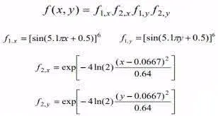
• To calculate f we have formulas.
• We are give a function called 'ga' which is genetic algorithm an inbuilt function in MATLAB.
• We are defining two variables in the function so the order will be 2 in the function.

FUNCTION CODE IN MATLAB:

% stalgamite function 
function [f]=stalagmite(input_vector)

x=input_vector(1);
y=input_vector(2);
f1_x=(sin(5.1.*pi.*x+0.5)).^6;
f2_y=(sin(5.1.*pi.*y+0.5)).^6;
f3_x=exp(-4*log(2).*(x-0.0667)^2/0.64);
f4_y=exp(-4*log(2).*(y-0.0667)^2/0.64);
f=-(f1_x.*f2_y.*f3_x.*f4_y);
end

• Above is the code for stalagmite function with two variables x and y.
• Generally 'ga' in Matlab gives us only the minimum value.
• But our intrest is to find the maximum value,so we are using a negative value for the value of f.

NOTE:While you find a lot of tools to minimize a function F, you find no functions to maximize F. Fortunately you can minimize G = -F, such that you do not need to program your own maximization tool.

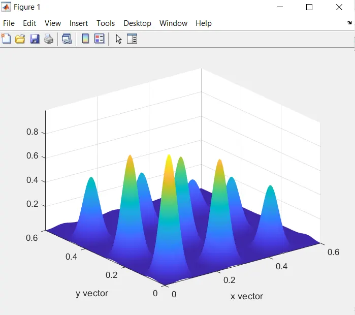
PROGRAM TO CALCULATE FOR THE DIFFERENT ITERATIONS:

STATISTICAL STUDY WITHOUT BOUNDATION:

%study 1 is for statistical behaviour
for i=1:num_cases
    [results,fopt(i)]=ga(@stalagmite,2);
    xopt(i)=results(1);
    yopt(i)=results(2);
end

study_time=toc

figure(1)
subplot(2,1,1)
hold on
surfc(x,y,-f)
shading interp

plot3(xopt,yopt,-fopt,'marker','o','markersize',5,'markerfacecolor','r')
xlabel('x value')
ylabel('y value')
title('unbounded inputs')
hold on
subplot(2,1,2)
plot(-fopt)
xlabel('iterations')
ylabel('function maximum')

• In this evaluation the optimum value of fitness function for each iteartion and calculating it by above syntax.
• Here we are taking 50 values which means 50 cases.
• By using tic toc command we can find the study time of the function.
• fopt will give the optimum values of x and y for each iteration.Negative sign is taken because our intrest is to find the maximum value.
• plotting all the values and making the subplot we get the plot of ga and the iterations.
• surf command is used to create a surface to visualize.
• Marker o is used to find the local maxima.

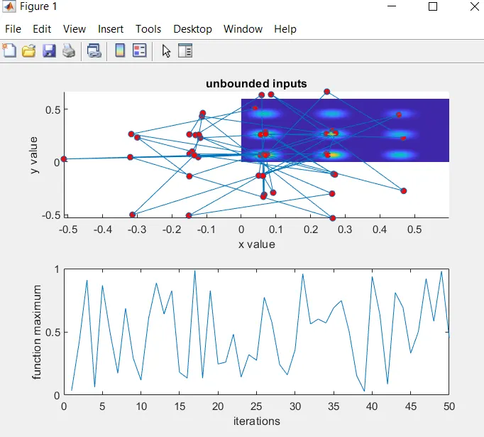
• from the graph it is observed that the inputs are unbounded and the results are not that much accurate and the value of iterations are changing.

STATISTICAL STUDY WITH BOUNDED INPUTS:

%study 2 is for statistical behaviour
for i=1:num_cases
    [results,fopt(i)]=ga(@stalagmite,2,[],[],[],[],[0;0],[0.6;0.6]);
    xopt(i)=results(1);
    yopt(i)=results(2);
end

study_time=toc

figure(2)
subplot(2,1,1)
hold on
surfc(x,y,-f)
shading interp
plot3(xopt,yopt,-fopt,'marker','o','markersize',5,'markerfacecolor','r')
xlabel('x value')
ylabel('y value')

title('bounded inputs')
hold on
subplot(2,1,2)
plot(-fopt)
xlabel('iterations')
ylabel('function maximum')

• As the above study is not accurate we are doing a second study with bounded inputs.
• In the we are setting a boundary limit for the ga so that the search page is reduced and the value of x and y are reduced.
• The syntax for this study is [results,fopt(i)]=ga(@stalagmite,2,[],[],[],[],[0;0],[0.6;0.6])
• Here, @stalagmite defines function,2 defines number of variables; [] define inequality and equality constraints;[0;0] defines lower boundary;[0.6;0.6]defines upper boundary.
• Same procedure is followed as above for remaining code.

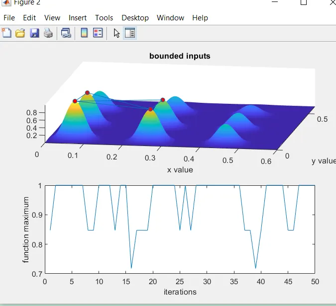
• From thr graph we observe that the upper limit is 0.6 and the graph is much clear than above case.
• Even this is not given us the exact result as the maximum values are at 4 points.
• To get only maximum value we are intrested in doing another study.

STATISTICAL STUDY WITH BOUNDED INPUTS WITH INCREASE IN POPULATION SIZE:

%study 3 is for statistical behaviour
for i=1:num_cases
    [results,fopt(i)]=ga(@stalagmite,2,[],[],[],[],[0;0],[0.6;0.6],[],[],options);
    xopt(i)=results(1);
    yopt(i)=results(2);
end

study_time=toc

figure(3)
subplot(2,1,1)
hold on
surfc(x,y,-f)
shading interp
plot3(xopt,yopt,-fopt,'marker','o','markersize',5,'markerfacecolor','r')
xlabel('x value')
ylabel('y value')

title('bounded inputs with increase in population size')
hold on
subplot(2,1,2)
plot(-fopt)
xlabel('iterations')
ylabel('function maximun')

• In this study we are using 'optimoptions' command to increase the population size and increase the probability of getting the maximum value.
• The advantage of this command is it will be working on large set of numbers and possibility to get the better fitness in the function.
• The syntax is [results,fopt(i)]=ga(@stalagmite,2,[],[],[],[],[0;0],[0.6;0.6],[],[],options)
• Rest of the code is same as the above cases.

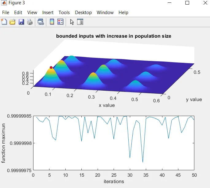
From the graph we can observe that the there is only one maximum point.

FUNCTION CODE:

% stalgamite function 
function [f]=get_stalagmite(x,y)

f1=(sin((5.1*pi.*x)+0.5)).^6;
f2=(sin((5.1*pi.*y)+0.5)).^6;
f3=exp((-4*log(2).*((x-0.0667).^2))/(0.64));
f4=exp((-4*log(2).*((y-0.0667).^2))/(0.64));
f=-(f1.*f2.*f3.*f4);
end

COMPLETE CODE:

clear all 
close all
clc


x=linspace(0,0.6,150);
y=linspace(0,0.6,150);
num_cases=50;
[x,y]=meshgrid(x,y);

tic
f=get_stalagmite(x,y);
%study 1 is for statistical behaviour
for i=1:num_cases
    [results,fopt(i)]=ga(@stalagmite,2);
    xopt(i)=results(1);
    yopt(i)=results(2);
end

study_time=toc

figure(1)
subplot(2,1,1)
hold on
surfc(x,y,-f)
shading interp

plot3(xopt,yopt,-fopt,'marker','o','markersize',5,'markerfacecolor','r')
xlabel('x value')
ylabel('y value')
title('unbounded inputs')
hold on
subplot(2,1,2)
plot(-fopt)
xlabel('iterations')
ylabel('function maximum')


tic

%study 2 is for statistical behaviour
for i=1:num_cases
    [results,fopt(i)]=ga(@stalagmite,2,[],[],[],[],[0;0],[0.6;0.6]);
    xopt(i)=results(1);
    yopt(i)=results(2);
end

study_time=toc

figure(2)
subplot(2,1,1)
hold on
surfc(x,y,-f)
shading interp
plot3(xopt,yopt,-fopt,'marker','o','markersize',5,'markerfacecolor','r')
xlabel('x value')
ylabel('y value')

title('bounded inputs')
hold on
subplot(2,1,2)
plot(-fopt)
xlabel('iterations')
ylabel('function maximum')


tic

options=optimoptions('ga')
options=optimoptions(options,'populationsize',170)


%study 3 is for statistical behaviour
for i=1:num_cases
    [results,fopt(i)]=ga(@stalagmite,2,[],[],[],[],[0;0],[0.6;0.6],[],[],options);
    xopt(i)=results(1);
    yopt(i)=results(2);
end

study_time=toc

figure(3)
subplot(2,1,1)
hold on
surfc(x,y,-f)
shading interp
plot3(xopt,yopt,-fopt,'marker','o','markersize',5,'markerfacecolor','r')
xlabel('x value')
ylabel('y value')

title('bounded inputs with increase in population size')
hold on
subplot(2,1,2)
plot(-fopt)
xlabel('iterations')
ylabel('function maximun')

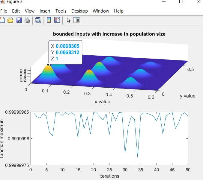
The maximum value is seen on the graph and the value of x,y,z are shown

ERRORS:

The = value is replaced by another by underscore

x'y is replaced by x'y

REFERENCES:

https://in.mathworks.com/matlabcentral/answers/52240-how-to-find-max-fuction-with-genetic-algorithm

https://www.mathworks.com/matlabcentral/answers/446830-how-would-i-get-maximization-curve-in-ga-in-matlab