Week 4 - Genetic Algorithm

Project:- code in MATLAB to optimize the stalagmite function and find the Global Maxima

In order to deal with a Genetic Algorithm, we need to under some of its basic concepts like

• What is Optimisation?

• What are all the techniques available to perform optimization?

• What is GA?

• How does GA Works?

• Where GA is used?

Learnings:- https://skill-lync.com/knowledgebase/genetic-algorithm-explained

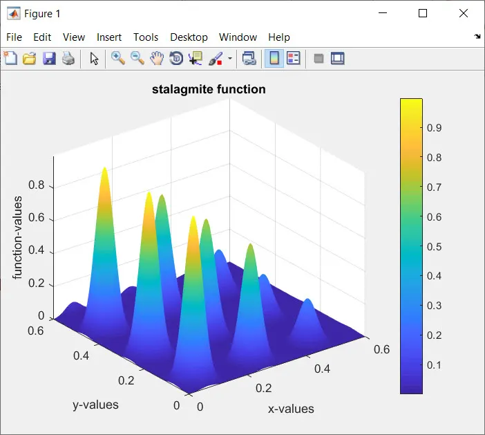
Stalagmite Function:-

• It's a mathematical model that helps us to generate the local minima's & maxima's
• we need to determine the global maximum of the function without prior to a particular field.
• In order to do that we need to optimize the data
• Firstly will define a function and later find the global maxima point

Genetic Algorithm:-

• Genetic Algorithm is based upon the evolution theory proposed by Charles Darwin.
• Matlab provides in-built functions in order to provide GA

Function Code:-

Defining the Stalagmite Function:-

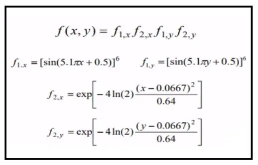
% Stagamite Function using the formula
function [f] = stalgamite_function(input_vector)
%consider
x = input_vector(1);
y = input_vector(2);

%therefore

f1x = (sin(5.1*pi*x + 0.5))^6;
f1y = (sin(5.1*pi*y + 0.5))^6;
f2x = exp(-4*log(2)*(x - 0.0667)^2/0.64);
f2y = exp(-4*log(2)*(x - 0.0667)^2/0.64);

f = -(f1x*f1y*f2x*f2y);
end

Actual Main Code:-

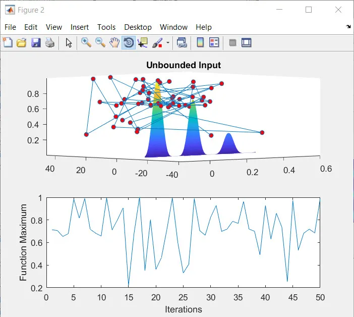
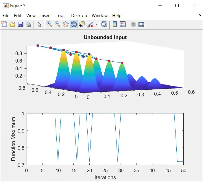
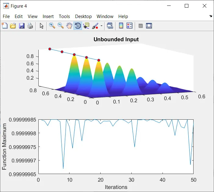
Plotting graphs for all 3 studies and for F maximum vs no. of iterations:-

• x,y are input array's.
• Alorithm is runned up to 50 times.
• %study 1 defining the ga
• figure window with sub-plots
• surfc(x,y,f) & plot3 command to visualize the optimum value that ga predicts over the 50 studies
• Another sub plot defines the optimum value that the function is predicting as the function of iteration
• tic & toc commands are used to evaluate the time taken for study1
• similarly other studies are carried out changing the samples
• X-axis is Iterations & Y-axis is Function Maxima Values.

x = linspace(0,0.6,150);
y = linspace(0,0.6,150);
num_iteration = 50

[xx yy] = meshgrid(x,y);

for  i = 1:length(xx)
    for j = 1:length(yy)
        input_vector(1) = xx(i,j);
        input_vector(2) = yy(i,j);
        f(i,j) = stalgamite_function(input_vector);
    end
end
figure
surfc(x,y,-f)
colorbar
xlabel('x-values')
ylabel('y-values')
zlabel('function-values')
title('stalagmite function')
shading interp

[x_output , fval] = ga(@stalgamite_function,2)

%Study 1 - Statistical Behaviour
tic
for i = 1:num_iteration
    [inputs , fopt(i)] = ga(@stalgamite_function,2);
    xopt1(i) = inputs(1);
    yopt1(i) = inputs(2);
end
Study1_Timing = toc
figure
subplot(2,1,1)
hold on
surfc(x,y,-f)
shading interp
plot3(xopt1,yopt1,-fopt,'marker','o','markersize',5,'markerfacecolor','r')
title('Unbounded Input')
subplot(2,1,2)
plot(-fopt)
xlabel('Iterations')
ylabel('Function Maximum')
%Study 2 - Statistical Behaviour- With upper and Lower Bounds
tic
for i = 1:num_iteration
    [inputs , fopt(i)] = ga(@stalgamite_function,2,[],[],[],[],[0;0],[1;1]);
    xopt2(i) = inputs(1);
    yopt2(i) = inputs(2);
end
Study2_Timing = toc
figure
subplot(2,1,1)
hold on
surfc(x,y,-f)
shading interp
plot3(xopt2,yopt2,-fopt,'marker','o','markersize',5,'markerfacecolor','r')
title('Unbounded Input')
subplot(2,1,2)
plot(-fopt)
xlabel('Iterations')
ylabel('Function Maximum')
%Study 3 - increasing ga iterations
options = optimoptions('ga')
options = optimoptions(options , 'populationsize', 200)
tic
for i = 1:num_iteration
    [inputs , fopt(i)] = ga(@stalgamite_function,2,[],[],[],[],[0;0],[1;1],[],[],options);
    xopt3(i) = inputs(1);
    yopt3(i) = inputs(2);
end
Study3_Timing = toc
figure
subplot(2,1,1)
hold on
surfc(x,y,-f)
shading interp
plot3(xopt3,yopt3,-fopt,'marker','o','markersize',5,'markerfacecolor','r')
title('Unbounded Input')
subplot(2,1,2)
plot(-fopt)
xlabel('Iterations')
ylabel('Function Maximum')

Plottings for Global Maxima:-