Week 4 - Genetic Algorithm

Objective: To maximise the stalagmite function using Matlab's genetic algorithm function and find the maxima

Theory: Genetic algorithm uses the concept of evolution through natural selection to reach a global minima for a given function.

It uses a set of data points called the first generation as the basis for the first run. This population of points may or may not lead to the desired global minima. 

In the next run, the algorithm chooses the optimum points that are closest to reaching the minima, alongwith new random points and uses them as the population for the next runs.

In this way, the algorithm converges to a minima in a few runs.

The stopping condition is the conditions when the algorithm will stop the process and output the results.

This could be:

When a certain amount of runs have been carried out

When a certain amount of time has passed.

When the result from newer runs arent substantially better than the previous.

We will be using Genetic algorithm to maximise the given stalagmite function. To maximise, we will have to modify it so that the algorithm gives a maxima instead of the minima.

The stalagmite function is:

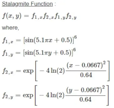
We need to maximise this using the GA function.

To do that, we will multiply the function by -1 to convert it to the negative domain.

This means the function now represents the inverted stalagmite function, and its minima will represent the maxima of the original stalagmite function

After we find the minima and the co-ordinates for a set of runs, we will plot them and multiply the results with -1 to get the actual value of the original stalagmite function.

We will use a for loop to run multiple iterations of the ga function to see how the global minimas are plotted for various populations.

We will use the following syntax which lets us specify the lower and upper bounds:

x = ga(function, nvars,A, b, Aeq, beq, lb, ub)

where x is the output, which can be customised from the ga options parameters. But for our example we will stick with the default set of outputs which is the x and y co-ordinates of the minima and the value of the minima.

nvars is the number of variables in the function.

A,b, Aeq and beq are matrices used to specify the linear equalities and inequalities. We wont use them for our case, so we will use empty brackets to denote them. 

Code: 

A. The inverted stalagmite function

function[op] = stalagmite(a)

%defining the 4 terms of the equation

f1 = (sin(5.1*3.14*a(1)+0.5));
f2 = (sin(5.1*3.14*a(2)+0.5));
f3 = exp(-4*log(2)*(((a(1)-0.06667)^2)/0.64));
f4 = exp(-4*log(2)*(((a(2)-0.06667)^2)/0.64));

%defining the output
op = -1*f1*f2*f3*f4;

end

B. Main program

clear all
close all
clc

%Generating the workspace
x = linspace(0,0.6,200);
y = linspace(0,0.6,200);

%using meshgrid to convert the linear workspace into a co-ordinate system
[X,Y] = meshgrid(x,y);

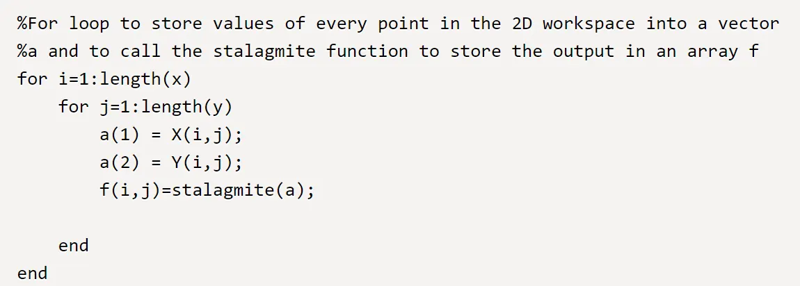
%For loop to store values of every point in the 2D workspace into a vector
%a and to call the stalagmite function to store the output in an array f
for i=1:length(x)
    for j=1:length(y)
        a(1) = X(i,j);
        a(2) = Y(i,j);
        f(i,j)=stalagmite(a);
        
    end
end


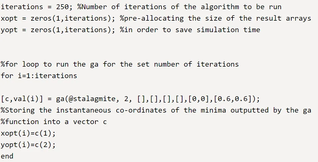
iterations = 250; %Number of iterations of the algorithm to be run
xopt = zeros(1,iterations); %pre-allocating the size of the result arrays
yopt = zeros(1,iterations); %in order to save simulation time


%for loop to run the ga for the set number of iterations
for i=1:iterations
    
[c,val(i)] = ga(@stalagmite, 2, [],[],[],[],[0,0],[0.6,0.6]);
%Storing the instantaneous co-ordinates of the minima outputted by the ga
%function into a vector c
xopt(i)=c(1); 
yopt(i)=c(2);
end


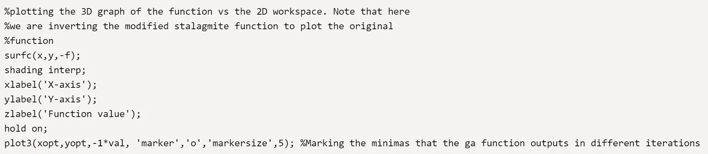
%plotting the 3D graph of the function vs the 2D workspace. Note that here
%we are inverting the modified stalagmite function to plot the original
%function
surfc(x,y,-f);
shading interp;
xlabel('X-axis');
ylabel('Y-axis');
zlabel('Function value');
hold on;
plot3(xopt,yopt,-1*val, 'marker','o','markersize',5); %Marking the minimas that the ga function outputs in different iterations

%Displaying the result
[maxval, ind] = max(-val); %since val is the minima of the modified stalagmite function we use -val to get the required max value.
result = ['The maximum value of the function is ', num2str(maxval), ' at co ordinates X = ', num2str(xopt(ind)), ' and Y = ', num2str(yopt(ind))];
disp(result);

Output:

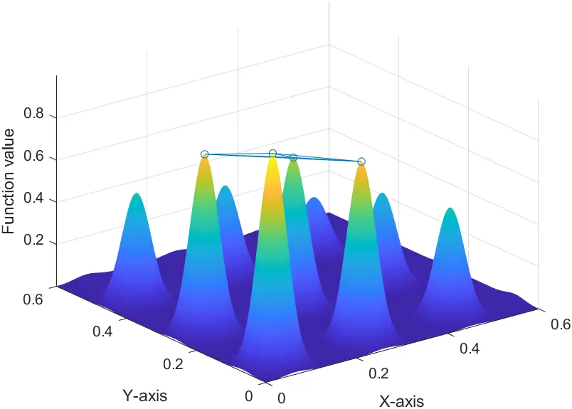
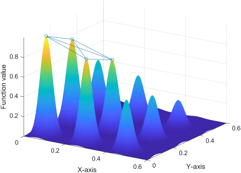
We can see that the ga function has returned 4 optimised values, out of which 1 is the global value and the rest are local.

Thus we can see that in some of the iterations the ga function has returned local value instead of the global value.

This is why we need to run ga function for multiple iterations to arrive at an accurate value.

Explanation:

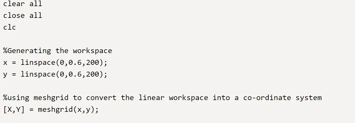
1. In the first step we create an array of numbers from 0 to 6 using linspace and then use meshgrid to create various combinations of them, to simulate the points of a 2D workspace

2. Then we use a nested for loop to call the stalagmite function for the above generated 2D workspace.

The results are stored in a function f

3. Then we define the number of iterations to be used for our ga algorithm. We also pre-allocate the size of the results array i.e xopt and yopt, so that the process is much faster.

Then we run the ga algorithm using a for loop. The results are stored in arrays c and val. c is the output array where the ga stores the co-ordinates of the minima for that particular instance. We copy these values into xopt and yopt for that instance. We are specifying lower and upper bounds in the ga function and hence we need to use empty brackets for the previous terms as per the syntax.

4. Next we plot the 3D graph ofthe function vs the 2D workspace. We plot -f as we had modified the function to be inverted, and now we need the original function.

We also mark the xopt and yopt and minimas outputted by the ga function here. We will be using -val for the same reason as using -f.

5. Lastly we will create an output showing the global maxima and its co-ordinates.

We use the max function to store the maximum of the -val array and its indices.

Then we display the maxima and use the indices to get the co-ordinates from the xopt and yopt values.

We have to use num2str function here to diplay the value of the variables.