Week 4 - Genetic Algorithm
Genetic Algorithm Program to find the maxima of a Stalagmite Function
Genetic Algorithm is high level procedure used in computer science, which is primarily used for generating superior quality solutions for any given problem undergoing an optimization process. As the name suggests, this algorithm relies on the basics of genetics in living organisms, where every new generation will evolve newer features, keep useful features and discard obsolete features so that the organism will have the capability to thrive in the ever changing living conditions. The same concept is used by genetic algorithm, where a sample (population) is evolved to better solutions using biologically inspired actions such as mutation and selection.
The algorithm works by evaluating the population for its fitness, with the fitness being evaluated by comparing the objective function to the value of every individual. The algorithm determines which individuals have their value closest to the objective function and selects them (selection operator). Then the crossover of data is initiated where the favourable set of data is merged with another set of data to create new data that can yeild better results (crossover operator). The selected individuals are modified and represented as the next generation (mutation operator). This is done to maintain diversity and to avoid convergence of data too early. In the next iteration, these new individuals are then compared again with the objective function.
This process goes on till the optimum solution is reached. The algorithm terminates either when the fitness is reached or when the maximum nunber of iterations are reached. The higher the number of iterations or the population size, the higher will be the accuracy of the algorithm's output.
In MATLAB, the genetic algorithm solver is denoted by the syntax 'ga', and it only calculates the minimum of the function. To find the maxima, the function must be multiplied by -1, since the minima of y=-f(x) is the same as the maxima of f(x). The following syntaxes are the acceptable inputs for the ga solver in MATLAB:
1)x = ga(fun,nvars)
where, x = function minimum
fun = objective function
nvars = no. of variables in objective function
This id the most basic form of the ga syntax, where it considers only the objective function and the variables within it as the parameters.
2)x = ga(fun,nvars,A,b)
This syntax now considers the inequality A*x`le`b, to which the function is subjected to. It considers linear inequality constraints as parameters. Must be left blank([]), if they don't exist.
3)x = ga(fun,nvars,A,b,Aeq,beq)
This syntax now considers the equality Aeq*x`le`beq, to which the function is subjected to. It considers linear equality constraints as parameters. Must be left blank([]), if they don't exist.
4)x = ga(fun,nvars,A,b,Aeq,beq,lb,ub)
This syntax considers the upper and lower bounds for the ga to consider. The ga will only search for solutions within the range specified by the parameters lb and ub, such that `lb le x le ub`. Must be left blank([]), if they don't exist.
5)x = ga(fun,nvars,A,b,Aeq,beq,lb,ub,nonlcon)
This syntax considers the a vector or array x and returns two arrays c(x) and ceq(x). Must be left blank([]), if they don't exist.
5)x = ga(fun,nvars,A,b,Aeq,beq,lb,ub,nonlcon,options)
This syntax replaces the default optimization parameters with custom parameters specified by the user.
Program:
The following program considers 3 cases:
1) Genetic Algorithm solution without considering boundary conditions
2) Genetic Algorithm solution considering boundary conditions
3) Genetic Algorithm solution considering boundary conditions and increased population size
Program Code:
%program to execute genetic algorithm function to optimise the solution
%for finding the minima of a given function

clear all
close all
clc

x = linspace(0,0.6,150);              %specifying the ranges in x and y direction for the search space to be considered by the ga function
y = linspace(0,0.6,150);

[xx,yy] = meshgrid(x,y);              %creating a 2D array using the 1D x and y values

for i=1:length(xx)
  for j=1:length(yy)
    input_vector(1) = xx(i,j);             %taking values from xx meshgrid
    input_vector(2) = yy(i,j);             %taking values from yy meshgrid
    f(i,j) = stlgfunc(input_vector);       %calling the function to evaluate the solution using the values of input_vector 1 & 2
  end
end

n=50;                                      %number of iterations(generations) to be considered by the ga solver

%study 1: no upper or lower boundary set
tic                                        %start of timer to calculate the time taken by the program to run the iterations
for i=1:n
[inputs,fopt(i)] = ga(@stlgfunc,2);        %ga solver called, with the function and number of variables specified
xopt(i) = inputs(1);                       %storing the new x values obtained for each iteration
yopt(i) = inputs(2);                       %storing the new y values obtained for each iteration
end
st_time_1 = toc                            %stopping the timer to show the time taken for the process

figure(1)
subplot(2,1,1)
hold on
surfc(xx,yy,-f)                            %creating the 3D surface using the meshgrid values and function
shading interp                             %specifying the surface requirement for the 3D surface
plot3(xopt,yopt,-fopt,'marker','o','markersize',4,'markerfacecolor','g')                 %plotting the function maxima according to the ga solver onto the surface
title('Genetic Algorithm solution obtained without boundary conditions')
xlabel('x values')
ylabel('y values')
subplot(2,1,2)
plot(-fopt)
xlabel('Iterations')
ylabel('Maxima')

%study 2: Upper and Lower boundary set
tic
for i = 1:n
    [inputs,fopt(i)] = ga(@stlgfunc,2,[],[],[],[],[0;0],[1;1]);     %specifying the lower and upper limits to the ga solver
    xopt(i) = inputs(1);
    yopt(i) = inputs(2);
end
st_time_2 = toc

figure(2)
subplot(2,1,1)
hold on
surfc(xx,yy,-f)
shading interp
plot3(xopt,yopt,-fopt,'marker','o','markersize',4,'markerfacecolor','g')
title('Genetic Algorithm solution obtained with boundary conditions')
xlabel('x values')
ylabel('y values')
subplot(2,1,2)
plot(-fopt)
xlabel('Iterations')
ylabel('Maxima')

%study 3: Boundaries set with increased population size
options = optimoptions('ga');
options = optimoptions(options,'PopulationSize',600);              %changing the default population(no. of samples)to 600
tic

for i = 1:n
    [inputs,fopt(i)] = ga(@stlgfunc,2,[],[],[],[],[0;0],[1;1],[],[],options);       %specifying the population,lower and upper limits to the ga solver
    xopt(i) = inputs(1);
    yopt(i) = inputs(2);
end
st_time_3 = toc

figure(3)
subplot(2,1,1)
hold on
surfc(xx,yy,-f)
shading interp
plot3(xopt,yopt,-fopt,'marker','o','markersize',4,'markerfacecolor','g')
title('Genetic Algorithm solution obtained with boundary conditions and increased population')
xlabel('x values')
ylabel('y values')
subplot(2,1,2)
plot(-fopt)
xlabel('Iterations')
ylabel('Maxima')
Function code:
function [f] = stlgfunc(input_vector)


f1x = (sin((5.1*pi).*input_vector(1)+0.5)).^6;
f1y = (sin((5.1*pi).*input_vector(2)+0.5)).^6;
f2x = exp(-4*(log(2))*(((input_vector(1)-0.0667).^2)./0.64));
f2y = exp(-4*(log(2))*(((input_vector(2)-0.0667).^2)./0.64));
f = -(f1x*f1y*f2x*f2y);
end
1) Study 1: Genetic Algorithm solution without considering boundary conditions
First, we specify the range in which the function and the surface is to be generated. The linspace command is used to divide the range of 0 to 0.6 into 150 parts and the values are stored in row vectors, for each x and y axes.
Next the meshgrid command is used to create two 2D grids, xx and yy. The grid will be used for plotting the surface along with the function.
After this, the for loop is utilised to pick each and every element from the xx and yy grids and calculate the solution for the function specified in the function code for those values of x and y. The following are the equations used in the function code:
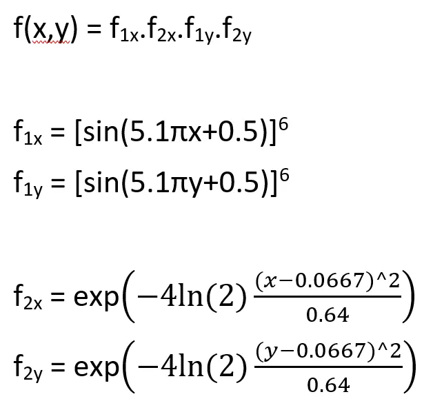
The no. of iterations (n) are set to 50.
For the first study, the boundary conditions are not set. First the 'tic toc' function is used to determine the time taken by the algorithm to run the 50 iterations. The for loop runs the 50 iterations. The ga solver is called within the loop, with the function code name (stlgfun) and the number of variables within that code (2) given as the solver's parameters. The output of the solver gives the inputs at which the function attains a maximum value (fopt). xopt and yopt are stored only when the ga solver finds a pair of x and y values which when put into the objective function gives the maximum value.
The figure is then created using the subplot function to add two plots within a single figure window. The first plot creates the 3D surface using the 'surfc' command which considers the values of xx,yy and the original function code's values for the corresponding xx and yy values. Shading interp is used to remove the grid lines on the 3D surface. plot3 command is used to plot points using the xopt,yopt and fopt in 3D space. The second subplot is used to show the variation of the maxima of the function with each iteration and considers the fopt values. The following plot is created:
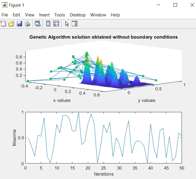
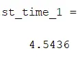
It is observed that the points predicted by the solver are all over the place, and the maxima varies from 0 to 1. The limitation of this study is that the ga solver is not given boundary conditions to work with, and hence considers values below 0 and above 0.6. This is solved in the next study, where the boundary conditions are set`
2) Study 2: Genetic Algorithm solution considering boundary conditions
The code for this study is same as that of the previous one, with the only exception being the input of the ga solver. Along with the function name and no. of variables, the lower and upper bounds are also specified (ga(@stlgfunc,2,[],[],[],[],[0;0],[1;1])). The inputs which are not required are left out by using empty square brackets. [0;0] specifies the lower bound and [1;1] specifies the upper bound.
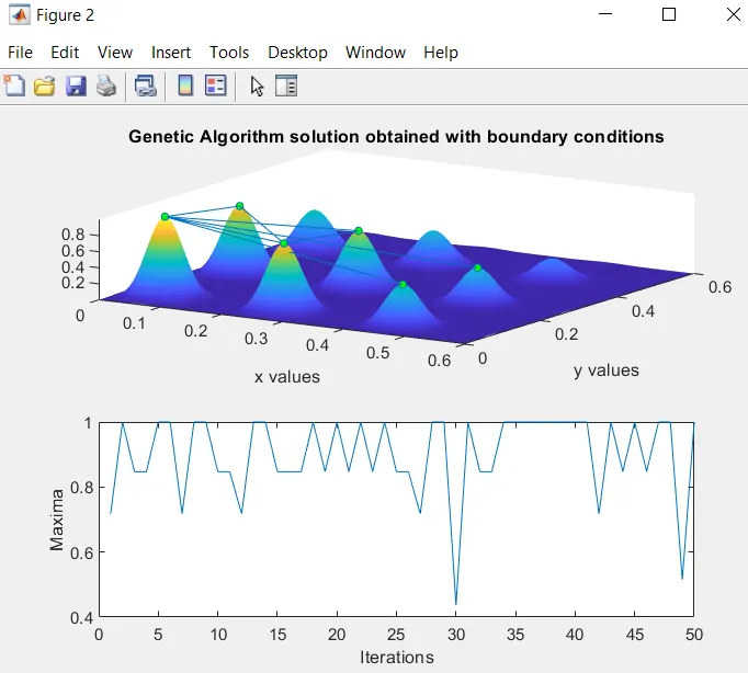
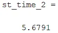
Here, it is observed that the plot is much cleaner. The boundary conditon eliminated unneccessary points. Also, the maxima now varies along a narrower range of 0.4 to 1. The time taken is also not much more than the previous study. The limitation is that the solver also considers local maxima along with the global maxima that is actually needed. Hence we modify the algorithm in the next study.
3) Study 3: Genetic Algorithm solution considering boundary conditions and an increased population
The ga solver in MATLAB always considers a set of values as its default value, including the population size. So to increase or modify the population size, the 'optimoptions' command is used. The purpose of this command is to modify any default values within the ga algorithm. The option is used to change the population size from the default 50 to 600. The advantage of increasing the population size is that it reduces the errors after every iteration. The large population will tend to shift the solution towards the more accurate answer.
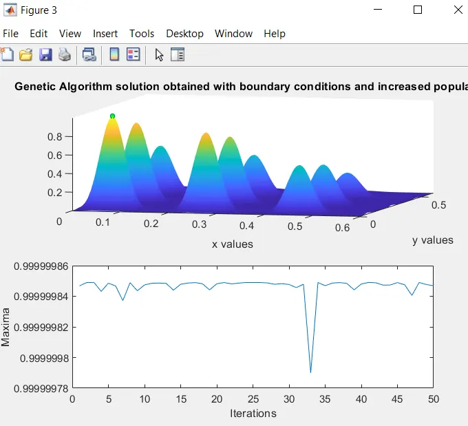
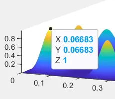
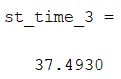
The 3rd study accurately predicts the global maxima as a singular point. The increased population helped in narrowing down the accurate result. The maxima also stays close to 1. But this process is very time consuming.
Conclusion:
From the 3 studies, it can be concluded that the Genetic Algorithm is an essential tool in obtaining optimum solutions for any engineering application. Highly optimised solutions for challenging problems can be readily obtained, which in turn optimises aspects within the industry such as time and cost savings, reduced wastage, improved designs etc.
References:
https://www.geeksforgeeks.org/genetic-algorithms/