Week 4 - Genetic Algorithm

AIM: To solve global maximum for a surface-plot using Matlab/Octave.

Objective:

To write a program to create a 2Dimensional Mesh for the inputs using meshgrid.

To write a program to perform optimization for a input data.

To check for the maximum value occured in the program.

Introduction:

Global optimization is a branch of applied mathematics and numerical analysis that attempts to find the global minima or maxima of a function or a set of functions on a given set.

Here, Optimization is the process of finding the point that minimizes a function. More specifically:

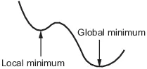
It is usually described as a minimization problem because the maximization of the real-valued

function is obviously equivalent to the minimization of the function .

Meshgrid:

The Meshgrid synatx is as follows : [xx, yy] = meshgrid(x,y);

Here, it returns a 2-D grid coordinates based on the coordinates contained in vectors x and y.

xx is a matrix where each row is a copy of x, and yy is a matrix where each column is a copy of y. The grid represented by the coordinates xx and yy has length(y) rows and length(x) columns.

In engineering problems, we need to consider some minimum values for a parameters that helps us to increase the efficiency of that problem, just like in piston cylinder we require minimum friction between surfaces, in airfoil we require minimum drag force etc.

We can get those minimum values by changing the surfaces and modifing the parameters but it takes a lot time and instead of doing all the process, the global optimization provides the require parameter by performing iterations.

Genetic Algorithm Syntax:

The genetic algorithm at the command line, call the genetic algorithm function 'ga' with the syntax
[x, fval] = ga(@fitness_func , ind_var, options);

where,
• @fitness_func is a handle to the fitness function.
• ind_var is the number of independent variables for the fitness function.
• options is a structure containing options for the genetic algorithm. If you do not pass in this argument, ‘ga’ uses its default options.

The results are given by,
• x — Point at which the final value is attained
• fval — Final value of the fitness function

There are more syntax available for genetic algorithm:

1. x= ga(fun,nvars)

Explanation/ Steps to follow:

To create the program initially; clear all, close and clc command should be used.

It is not mandatory but it is a good to clear the command window and workspace and the different windows of the software, so that you program looks clean and clear also closing the different unnessary windows helps to run the software smoothly.

Start with writing the starting points of the links and ending points of the links, so that you will not have a writing all the things at a same time.

It is always a good practice to write the program in small sections and checking for the errors and afterwards combine them together.

Now, we will write the codes for our stalgamite function as it is given in the video section.Note, here we did not need to write the clc, clear all and close all. As it is a sub-function and it is called from the main program and we did not want to clear the calculated data of the main program during calling this function.

Here, we are just attaching a minus at last of the stalagmite function.

Because, we want to calculate maximum value of the given function.

Now, after that we will go in our main program again.

Then we will create an array for x values and y values using linspace command.

Then we have to create a 2Dimensional mesh using x and y values and using meshgrid command.

Then we will create a inputs for our stalagmite function and using for loops we create a input vector for our stalagmite.

Then, we will run the genetic algorithm to solve the stalagmite function and evaluate our maximum value. After running this we will get only the plot, we would not get the maximum value.

So,after that we will run different studies for our program to calculate the maximum value.

In study-1, we will use the num_cases to do iterations and calculate the maximum value for the iterations upto 50.

Now,After running the program we might get the global maximum value but running the program again again, we will get various maximum values because, here we are getting local maximas too.

So, we need to bound the inputs in the stalagmite function so that we can get the values in a certain limit.

So, in study-2, we will define some inputs and while defining the inputs as we have no inequalities, so we will use empty square brackets, so that the program can know, there is no equalities.

Now, we still get the results in a bound region but still we didn't get the accurate results.

So, in the third study we will put some options in our code and will increase the Population size, this will results in more accurate results.

Now, we will get the plots according to the result.

Program:

1.Program to write a Stalagmite Function that is require to create local maxima and minima.

%Program to write a Stalagmite Function which is used to create local maxima and minima.
 
function [f] = stalagmite(inputs);
  
  %Getting input values of x and y from the main program 
  x = inputs(1);
  y = inputs(2);
  
  fx1 = [sin((5.1*pi*x)+ 0.5)]^6;
  fx2 = exp(-4*log(2)*(((x-0.0666)^2)/0.64));
  fy1 = [sin((5.1*pi*y)+ 0.5)]^6;
  fy2 = exp(-4*log(2)*(((y - 0.0666)^2)/0.64));
  f = -(fx1*fx2*fy1*fy2);
  
end

Here, we have defined the stalagmite function, now we will write our main program to use this stalagmite function to know the maximum value from the function.

2.Main Program to call a Stalagmite Function and evaluate the maximum value without upper and lower bounds.

%Program to find the maximum value (without upper and lower bounds) using Matlab/Octave

clear all
close all
clc

%Load the Genetic Algorithm Package
pkg load ga
pkg load optim

%Here, it creates an 1-Dimensional Arrays for x and y.
x = linspace(0,0.6,150);
y = linspace(0,0.6,150);

%Creating a 2D Mesh from 1-D array.
[xx yy] = meshgrid(x,y);
%Here, xx is a matrix where each row is a copy of x
%Whereas, yy is a matrix where each row is a copy of y.
%Grid has a X-coordinates of length(y) rows and Y-coordinates of length(x) column 

for i = 1:length(xx)
  for j = 1:length(yy)
    input_vector(1) = xx(i,j);
    input_vector(2) = yy(i,j);
    f(i,j) = stalagmite(input_vector);
  end
end

%To solve the genetic algorithm and get the global minima.
[inputs,fval] = ga(@stalagmite,2);

%Iterations to be Perform:
num_cases = 50;




%Study-1: Unbounded Inputs 
tic
for i = 1:num_cases;
  %To solve the genetic algorithm and get the global minima.  
  [inputs,fopt(i)]= ga(@stalagmite,2);
  xopt(i) = inputs(1);
  yopt(i) = inputs(2);
end
Study1_time = toc
%Plotting Study-1. 
figure(1);
%Creating a subplot within a plot
subplot(2,1,1);
hold on
%Surface Plot
surfc(xx,yy,f)
shading interp
%Marking points on the surface plot
plot3(xopt,yopt,fopt,'marker', 'o','markersize',5,'markerfacecolor','r')
title('Unbounded Inputs')
subplot(2,1,2)
%Plotting the negaative of the results
plot(fopt);
xlabel('iterations');
ylabel('function Maximum');

Results:

Here, the global maximum value are not only evaluated instead it gives the values for all the local maximum values too.

3.Program to call a Stalagmite Function and evaluate the maximum value (including upper and lower bounds.)

%Program to find the maximum value (without upper and lower bounds) using Matlab/Octave

clear all
close all
clc

%Load the Genetic Algorithm Package
pkg load ga
pkg load optim

%Here, it creates an 1-Dimensional Arrays for x and y.
x = linspace(0,0.6,150);
y = linspace(0,0.6,150);

%Creating a 2D Mesh from 1-D array.
[xx yy] = meshgrid(x,y);
%Here, xx is a matrix where each row is a copy of x
%Whereas, yy is a matrix where each row is a copy of y.
%Grid has a X-coordinates of length(y) rows and Y-coordinates of length(x) column 

for i = 1:length(xx)
  for j = 1:length(yy)
    input_vector(1) = xx(i,j);
    input_vector(2) = yy(i,j);
    f(i,j) = stalagmite(input_vector);
  end
end

%To solve the genetic algorithm and get the global minima.
[inputs,fval] = ga(@stalagmite,2);

%Iterations to be Perform:
num_cases = 50;

%Study-2 : Staticstical Behaviour with lower and upper bounds
tic
for i = 1:num_cases;
  %To solve the genetic algorithm and get the global minima.  
  [inputs,fopt(i)] = ga (@stalagmite,2,[],[],[],[],[0;0],[1;1]);
  xopt(i) = inputs(1);
  yopt(i) = inputs(2);
end
Study2_time = toc
%Plotting Study-1. 
figure(2);
%Creating a subplot within a plot
subplot(2,1,1);
hold on
%Surface Plot
surfc(xx,yy,f)
shading interp
%Marking points on the surface plot
plot3(xopt,yopt,fopt,'marker', 'o','markersize',5,'markerfacecolor','r')
title('UnBounded Inputs')
subplot(2,1,2)
plot(fopt);
xlabel('iterations');
ylabel('function Maximum');

Output:

Here, due to upper and lower bounds, it evaluates our maximum value in between these bounds only, and we get a maximum value from a definite range only.

Still, we are getting more number of maximas, so to get to an maximum value, we need to increase our iterations, so that we can get to maxima values more accurately.

4.Program to call a Stalagmite Function and evaluate the maximum value (including upper and lower bounds with increasing Population Size.)

%Program to find the maximum value (without upper and lower bounds) with increasing Population Size using Matlab.

clear all
close all
clc

%Load the Genetic Algorithm Package
pkg load ga
pkg load optim

%Here, it creates an 1-Dimensional Arrays for x and y.
x = linspace(0,0.6,150);
y = linspace(0,0.6,150);

%Creating a 2D Mesh from 1-D array.
[xx yy] = meshgrid(x,y);
%Here, xx is a matrix where each row is a copy of x
%Whereas, yy is a matrix where each row is a copy of y.
%Grid has a X-coordinates of length(y) rows and Y-coordinates of length(x) column 

for i = 1:length(xx)
  for j = 1:length(yy)
    input_vector(1) = xx(i,j);
    input_vector(2) = yy(i,j);
    f(i,j) = stalagmite(input_vector);
  end
end

%To solve the genetic algorithm and get the global minima.
[inputs,fval] = ga(@stalagmite,2);

%Iterations to be Perform:
num_cases = 5;

%Study-3 : Increasing GA studies
options = gaoptimset('PopulationSize',120);

tic
for i = 1:num_cases;
  %To solve the genetic algorithm and get the global minima.  
  [inputs,fopt(i)]= ga(@stalagmite,2,[],[],[],[],[0;0],[1;1],[],[],options);
  xopt(i) = inputs(1);
  yopt(i) = inputs(2);
end
Study3_time = toc
%Plotting Study-3. 
figure(3);
%Creating a subplot within a plot
subplot(2,1,1);
hold on
%Surface Plot
surfc(xx,yy,f);
shading interp
%Marking points on the surface plot
plot3(xopt,yopt,fopt,'marker', 'o','markersize',5,'markerfacecolor','r')
title('Increasing Iterations')
subplot(2,1,2);
plot(fopt);
xlabel('iterations');
ylabel('function Maximum');

Output:

Here, we still not get to a maximum value but it has given a feasible solution for our problem.

Increaing more iterations will give us more accurate result.

Thus, we can get the maximum value with the help of this program.

The results differs using Octave and Matlab software.

Actually, i have tried this program running at both the softwares, the plots are very different from the plots obtained in the matlab.

It is recommended to use the MATLAB software for this program only.

The errors obtain in octave are, the study-1 and study-2 has the same plots, the input bounds didn't work accurately.

Also, for study-3, the optimset package is not updated, it does not work properly, even in it's latest version.

Thank you for reading this out.