Genetic Algorithm in MATLAB

Objective

Write a code in MATLAB to optimise the stalagmite function and find the global maxima of the function.

Problem Statement

• Clearly expalin the concept of genetic algorithm in your own words and also explain the syntax for ga in MATLAB in your report.
• Make sure that your code gives the same output, even if it is made to run several times.
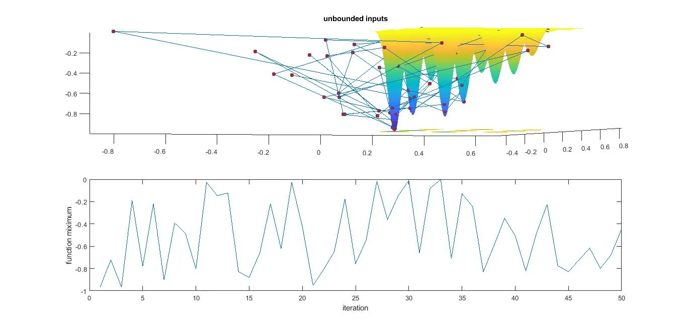
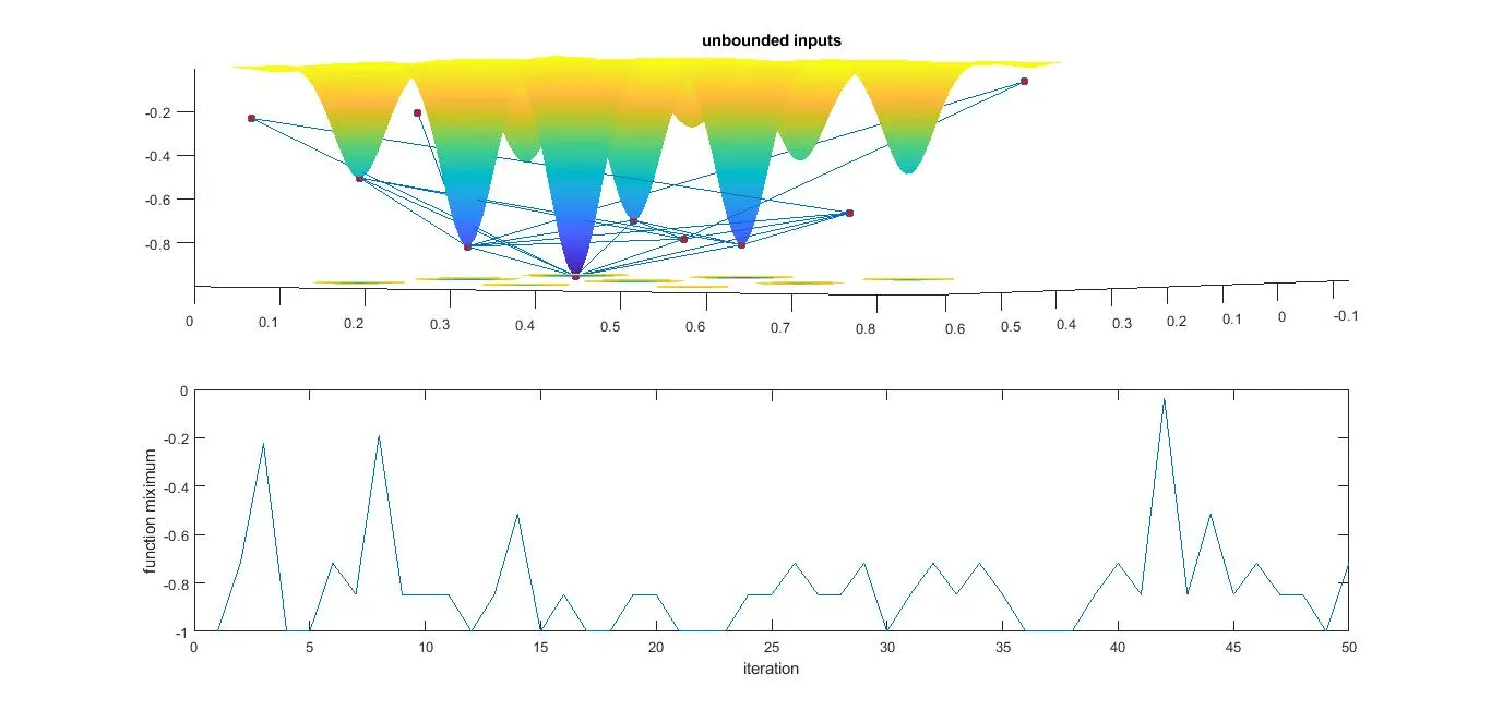
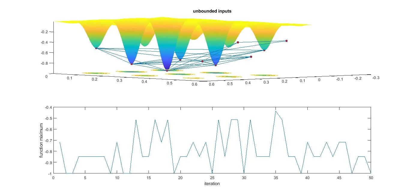
• Plot graphs for all 3 studies and for F maximum vs no. of iterations. Title and axes labels are a must, legends could be shown if necessary.

Theory

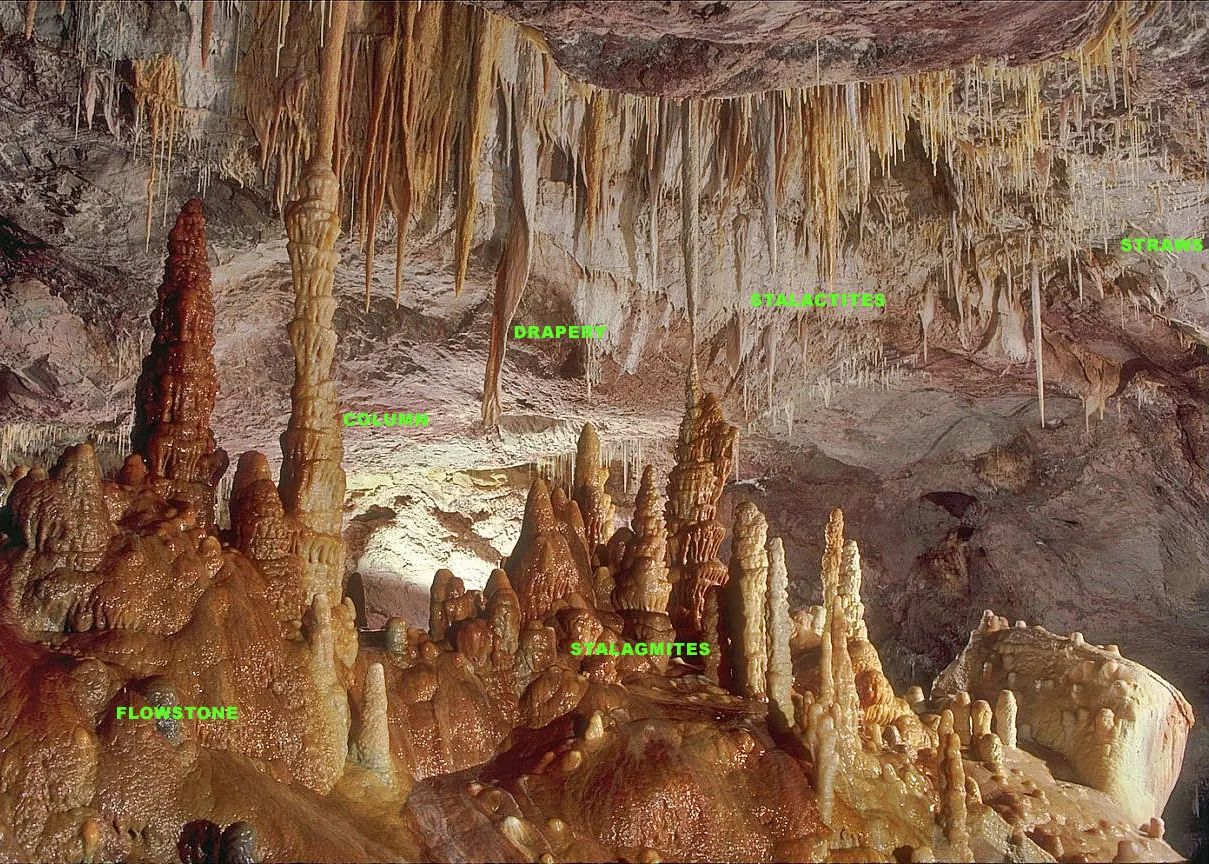
A stalagmite is an upward-growing mound of mineral deposits that have precipitated from water dripping onto the floor of a cave. Most stalagmites have rounded or flattened tips.

GENETIC ALGORITHM

close all
clear all
clc

%defining our search space
%one dimension
x=linspace(0,0.6,150);
y=linspace(0,0.6,150);
num_cases=50
%2 dimension
[xx yy]=meshgrid(x,y);
%evaluating the stalagmite function


for i=1:length(xx)
    for j=1:length (yy)
    input_vector(1)=xx(i,j);
    input_vector(2)=yy(i,j);
    f(i,j)=get_stalagmite(input_vector);
  
    end
end

%study_1 stastical behaviour

tic
for i=1:num_cases
  [inputs,fopt(i)]=ga(@get_stalagmite,2)
  xopt(i)=inputs(1);
  yopt(i)=inputs(2);
end


figure (1) 
subplot(2,1,1)
hold on
surfc(xx,yy,f)
shading interp
plot3(xopt,yopt,fopt,'marker','o','markersize',5,'markerfacecolor','r')
title('unbounded inputs')
subplot(2,1,2)
plot(fopt)
xlabel('iteration')
ylabel('function miximum')

%bounding the values

tic
for i=1:num_cases
  [inputs,fopt(i)]=ga(@get_stalagmite,2,[],[],[],[],[0:0],[1:1])
  xopt(i)=inputs(1);
  yopt(i)=inputs(2);
end
study_time_2=toc;

figure (2)
subplot(2,1,1)
hold on
surfc(xx,yy,f)
shading interp
plot3(xopt,yopt,fopt,'marker','o','markersize',5,'markerfacecolor','r')
title('unbounded inputs')
subplot(2,1,2)
plot(fopt)
xlabel('iteration')
ylabel('function miximum')

%study_3 bounding the values and increasing population size
tic
for i=1:num_cases
  [inputs,fopt(i)]=ga(@get_stalagmite,2,[],[],[],[],[0:0],[1:1])
  xopt(i)=inputs(1);
  yopt(i)=inputs(2);
end
study_time_2=toc;

figure (3)
subplot(2,1,1)
hold on
surfc(xx,yy,f)
shading interp
plot3(xopt,yopt,fopt,'marker','o','markersize',5,'markerfacecolor','r')
title('unbounded inputs')
subplot(2,1,2)
plot(fopt)
xlabel('iteration')
ylabel('function miximum')

function stalagmite = get_stalagmite(input_vector)
  x = input_vector (1)
  y = input_vector (2)
  f1_x = (sin (5.1 * pi * x + 0.5)) .^ 6;
  f2_y = (sin (5.1 * pi * y + 0.5)) .^ 6;
  f3_x = exp ((-4 * 0.6931) .* (x - 0.0667) .^ 2 / (0.64));
  f4_y = exp ((-4 * 0.6931) .* (y - 0.0667) .^ 2 / (0.64));
  stalagmite = -(f1_x .* f2_y .* f3_x .* f4_y)
end

CODE EXPLANATION

close all
clear all
clc

%defining our search space
%one dimension
x=linspace(0,0.6,150);
y=linspace(0,0.6,150);
num_cases=50
%2 dimension
[xx yy]=meshgrid(x,y);
%evaluating the stalagmite function

for i=1:length(xx)
for j=1:length (yy)
input_vector(1)=xx(i,j); %creating z ases by taking input from xx and yy each point
input_vector(2)=yy(i,j);
f(i,j)=get_stalagmite(input_vector);

end
end

%study_1 stastical behaviour

tic %timer on
for i=1:num_cases
[inputs,fopt(i)]=ga(@get_stalagmite,2) %calculating time for creating figure1
xopt(i)=inputs(1);
yopt(i)=inputs(2);
end

figure (1) %figure creating command
subplot(2,1,1)
hold on
surfc(xx,yy,f)
shading interp
plot3(xopt,yopt,fopt,'marker','o','markersize',5,'markerfacecolor','r')
title('unbounded inputs')
subplot(2,1,2)
plot(fopt)
xlabel('iteration')
ylabel('function miximum')

%bounding the values

tic
for i=1:num_cases %timer on
[inputs,fopt(i)]=ga(@get_stalagmite,2,[],[],[],[],[0:0],[1:1]) %calculating time for creating figure1
xopt(i)=inputs(1);
yopt(i)=inputs(2);
end
study_time_2=toc;

figure (2) %figure creating command
subplot(2,1,1)
hold on
surfc(xx,yy,f) %surface creating command
shading interp
plot3(xopt,yopt,fopt,'marker','o','markersize',5,'markerfacecolor','r')
title('unbounded inputs')
subplot(2,1,2)
plot(fopt)
xlabel('iteration')
ylabel('function miximum')

%study_3 bounding the values and increasing population size
tic %timer on
for i=1:num_cases
[inputs,fopt(i)]=ga(@get_stalagmite,2,[],[],[],[],[0:0],[1:1]) %calculating time for creating figure1
xopt(i)=inputs(1);
yopt(i)=inputs(2);
end
study_time_2=toc;

figure (3) %figure creating command
subplot(2,1,1)
hold on
surfc(xx,yy,f) %surface creating command
shading interp
plot3(xopt,yopt,fopt,'marker','o','markersize',5,'markerfacecolor','r')
title('unbounded inputs')
subplot(2,1,2)
plot(fopt)
xlabel('iteration')
ylabel('function miximum')

OUTPUT