Week 4 - Genetic Algorithm

AIM: Write a code in MATLAB to optimise the stalagmite function and find the global maxima of the function

THEORY:

Genetic Algorithm is a stochastic, population-based algorithm that searches randomly by mutation and crossover among populations. It helps solving smooth or non-smooth optimiztion problems with any types of constraints, including integer constraints.

It follows a set of stages -

1) Initialization - An array of numbers are defined as the initial population

2) Fitness function - This function defines the probability of a number in the population likely to be selected

3) Selection - It is the most fit number that has the highest probability of being selected for reproduction

4) Crossover - It involves creating a new set of numbers from the selected parent population

5) Mutation - The algorithm creates mutation children by randomly changing the genes of individual parents

6) Termination - The algorithm terminates if the population has converged

Genetic Algorithm (GA) syntax -

CASE STUDY 1:

x = ga(@fun, nvars);

finds a local unconstrained minimum, "x", to the objective function, "fun". "nvars" is the dimension (number of design variables) of fun.

CASE STUDY 2:

x = ga(@fun, nvars, A, b, Aeq, beq, lb, ub);

defines a set of lower and upper bounds on the design variables, "x", so that solution is found in the range lb<=x<=ub

Set Aeq = [] and beq = [] if non-linear equalities exists

CASE STUDY 3:

x = ga(@fun, nvars, A, b, Aeq, beq, lb, ub, nonicon, Intcon, options);

Minimizes with the default optimization parameters replaced by values in options (Set non-Icon = [] if no non-linear constraints exists)

Create options using optimoptions

PROCEDURE:

1. First the new editor window is opened, the commands "clear all", "close all" and "clc" are used to clear the command window and the previously done programs
2. The aim of the program is commented using the "%" symbol on the top of the editor window
3. The program written is saved using the extension ".m"
4. The search space is defined using the linspace comand
5. Now we use meshgrid feature
6. The stalagmite function is then evaluated
7. Three different case studies are made to understand statistical behaviour of the genetic algorithm
8. Then the plots for each of these cases are done

PROGRAMS:

Stalagmite function -

%To evaluate stalagmite function (optimise maxima)
function [F] = stalagmite1(input_vector)
      
     x = input_vector(1);
     y = input_vector(2);
     
     f11 = (sin(5.1*pi*x + 0.5).^6);
     f12 = (sin(5.1*pi*y + 0.5).^6);
     f21 = exp(-4*log(2)*((x-0.0667).^2/0.64));
     f22 = exp(-4*log(2)*((y-0.0667).^2/0.64));
     F =-(f11.*f12.*f21.*f22);
end

Main program -

%Genetic algorithm programme
clear all 
close all
clc

%defining or search space
x = linspace(0, 0.6, 150);
y = linspace(0, 0.6, 150);
num_cases = 50;

%creating a 2-Dimensional grid
[xx yy] = meshgrid(x, y);

%evaluating the stalagmite function 
for i = 1:length(xx)
    for j = 1:length(yy)
        input_vector(1) = xx(i, j);
        input_vector(2) = yy(i, j);
        f(i, j) = stalagmite1(input_vector);
    end
end


tic
%study1 - statistical behaviour
for i = 1 : num_cases
   [inputs, fopt(i)] = ga(@stalagmite1, 2);
   xopt(i) = inputs(1);
   yopt(i) = inputs(2);
end
study1_time = toc

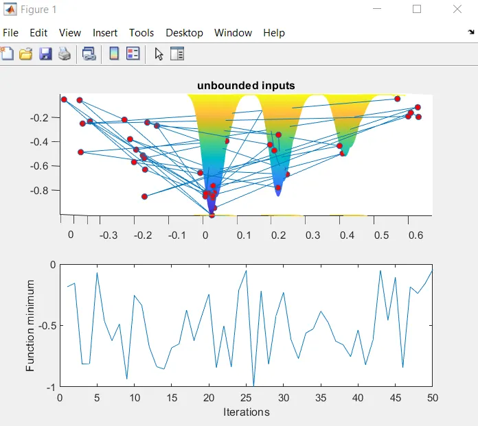
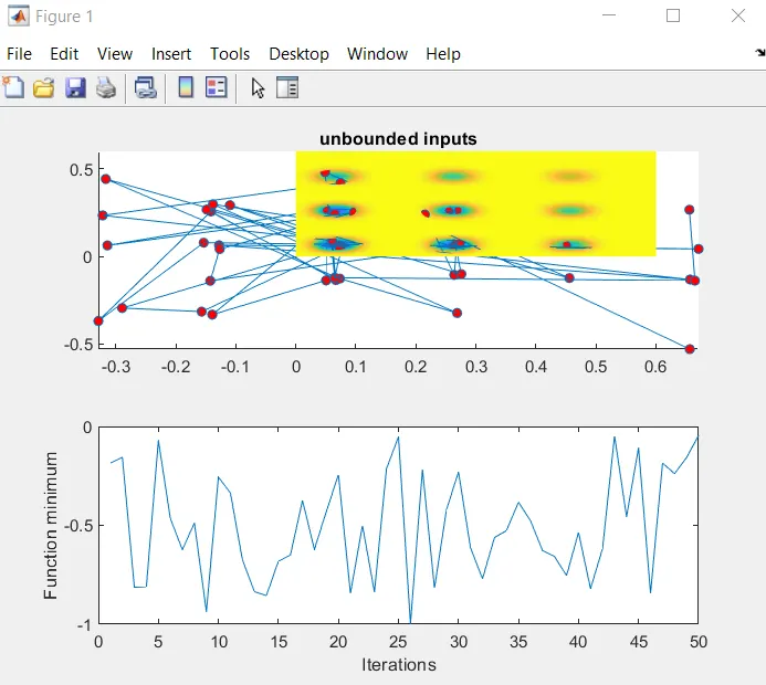
figure(1)
subplot(2, 1, 1)
hold on 
surfc(xx, yy, f)
shading interp
plot3(xopt, yopt, fopt, 'marker', 'o', 'markersize', 5, 'markerfacecolor', 'r')
title('unbounded inputs')
subplot(2, 1, 2)
plot(fopt)
xlabel('Iterations')
ylabel('Function minimum')

tic
%study 2 - statistical behaviour - with upper and lower bounds
for i = 1: num_cases
    
    [inputs, fopt(i)] = ga(@stalagmite1, 2, [], [], [], [], [0:0], [1:1]);
    xopt(i) = inputs(1);
    yopt(i) = inputs(2);
    
end
study2_time = toc

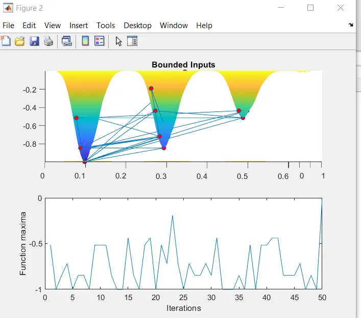
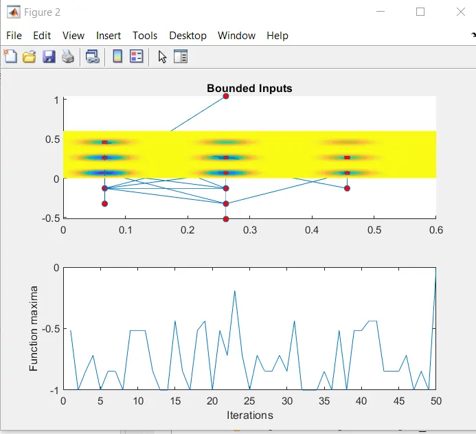
figure(2)
subplot(2, 1, 1)
hold on
surfc(xx, yy, f)
shading interp
plot3(xopt, yopt, fopt, 'marker', 'o', 'markersize', 5, 'markerfacecolor', 'r')
title('Bounded Inputs')
subplot(2, 1, 2)
plot(fopt)
xlabel('Iterations')
ylabel('Function maxima')

%study 3 - increasing GA iterations
options = optimoptions('ga');
options = optimoptions(options, 'PopulationSize', 150);

tic
for i = 1 : num_cases
    
    [inputs, fopt(i)] = ga(@stalagmite1, 2, [], [], [], [], [0:0], [1:1], [], [], options);
    xopt(i) = inputs(1);
    yopt(i) = inputs(2);
    
end
study3_time = toc
figure(3)
subplot(2, 1, 1)
hold on 
surfc(xx, yy, f)
shading interp
xlabel('x-axis');
ylabel('y-axis');
plot3(xopt, yopt, fopt, 'marker', 'o', 'markersize', 5, 'markerfacecolor', 'r')
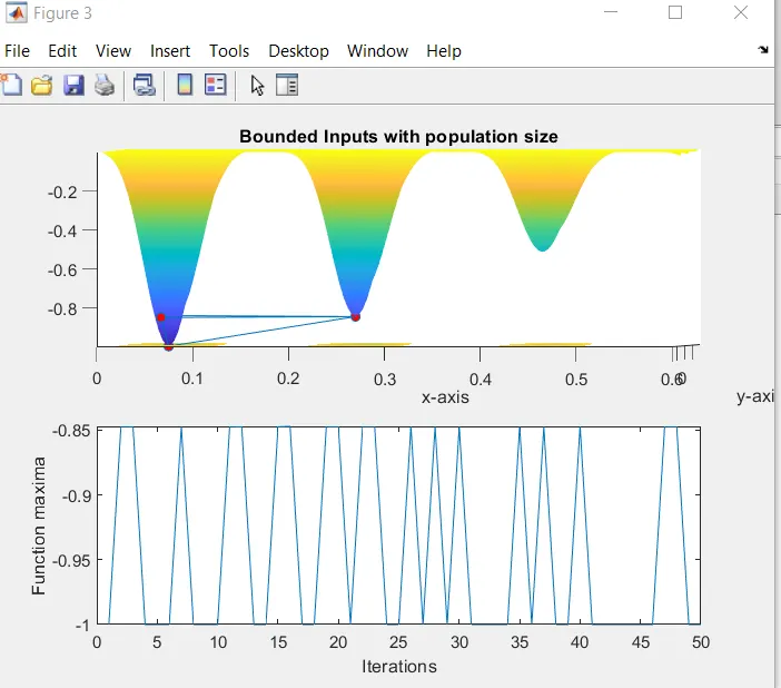
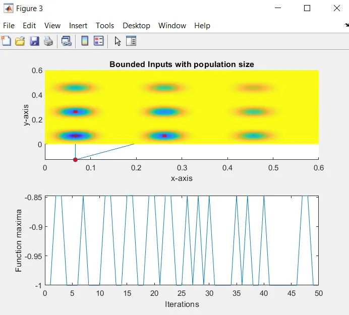
title('Bounded Inputs with population size')
subplot(2, 1, 2)
plot(fopt)
xlabel('Iterations')
ylabel('Function maxima')

[output, fval] = ga(@stalagmite, 2);
max_value = fopt;

PLOTS:

Plot with unbounded inputs in 3D and 2D format respectively

Plot with bounded inputs in 3D and 2D format respectively

Plot with bounded inputs and population size in 3d and 2D format respectively

ERRORS AND CORRECTION:

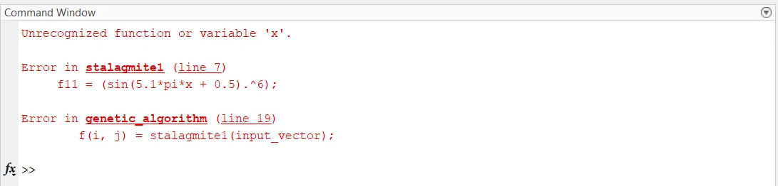
correction - inputs for x and y variables are given in the stalagmite function

EXPLANATION:

1. The meshgrid feature helps to create a grid for compatibility in evaluating the matrices, the vectors given in the meshgrid function will determine the order of the matrices
2. Stalagmite function helps to evaluate the maxima of the random values
3. Three different case studies are considered to get the value of maxima a) Using the degree of polynomial b) By giving a range, that is, Upper and lower bounds c) By considering a population size Plots are made and comparisons of different case studies are analysed

RESULTS:

Plots show that by considering the population size we can get an optimised maxima value.