Crash Box Simulation | LS-DYNA

AIM: To simulate a crash test for a crash box impacting on a rigidwall in LS-Dyna.

OBJECTIVES:

• To create a rigidwall in LS-Dyna on which the crash box can impact.
• To apply initial velocity of 50 kmph to the crash box.
• To run the simulation of crash box using two different thickness 1.2 mm and 1.5 mm respectively.
• To plot the cross-sectional force generated in the middle of the crash box.
• To plot and compare the accelerations and stress-strain plots of 1.2 mm and 1.5 mm crash boxes.

CASE SETUP:

A crash box is a highly energy absorbing structure that crashes on application of loads and reduces impact on other components nearby. A full-fledges crash box is a highly sophisticated design but in this case we will go with a rectangular channel which can thought of as the most simple crash box. The given rectangular crash box model is as shown below.

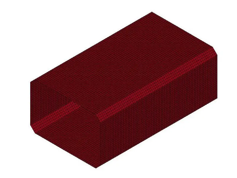
The crash box must impact on a rigid wall as per the crash requirement, so first we will create a rigidwall.

Rigidwall –

To create a planar rigidwall at one of the sides of the crash box, we will follow the procedure mentioned below.

• Go to Create Entity
• Under Rigidwall sub panel, go to Cre to create a new rigidwall.
• Select Planar option and under GeoVector select 1n+NL
• Select one of the nodes on the edge of the crash box. The rigidwall will then be created on the edges of the crash box so we will translate it by some distance so as to have space between the rigidwall and the crash box.
• Under GeoVector, select Trans option and translate the rigidwall by 15 mm in X-axis as shown below.

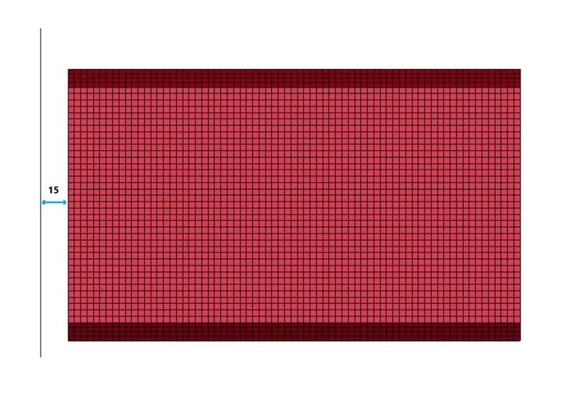
The rigidwall will be created as shown below.

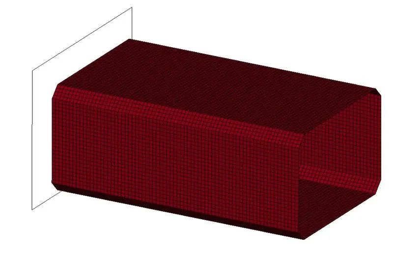
Initial Velocity –

The initial velocity of 50 kmph must be applied to the crash box in order to give translational motion to the crash box for impact with the rigidwall. So before creating the initial velocity keyword, we will create node set for all the shell elements of the crash box.

• Go to Create Entity
• Under Set Data sub panel, go to Cre to create a new *SET_NODE by selecting all the elements of the crash box.

Thus the node set for crash box is created. Now we will create Initial velocity keyword to impose velocity to the crash box elements.

• Go to Keyword Manager
• Select INITIAL > VELOCITY card and mention the node set ID which was created earlier.
• As we have to use gm-mm-ms unit system, we will provide initial velocity of -13.89 mm/ms (i.e. 50 kmph) in x-direction as shown below. Negative sign indicates that the velocity is applied in negative x-axis.

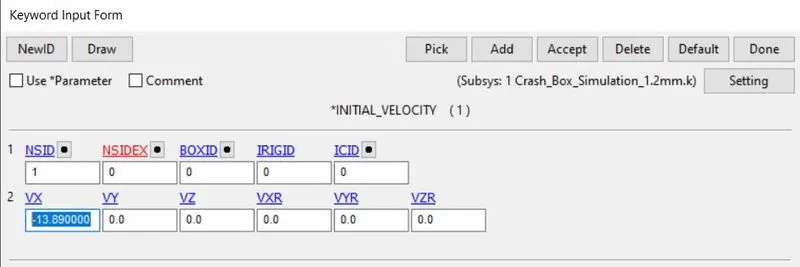
Thus the initial velocity is applied to the crash box.

Shell Section –

Shell section card is required to define section properties for shell elements.

• Go to Keyword Manager
• Select SECTION > SHELL Give it a section ID and title.
• Choose Element Formulation value in ELFORM as 2 which use Belytschko-Tsay type elements.
• Mention the thickness of the shell elements as 2 mm for one simulation and then 1.5 mm for the other simulation.

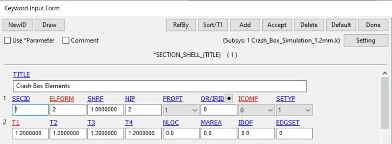
The Shell section card is ready.

Material –

For crash box, we will assign the material as steel which is a non-linear characteristic material.

• Go to Keyword Manager
• Select MAT > 024-PIECEWISE_LINEAR_PLASTICITY material card. Give it a material ID and title.
• As we are using gm-mm-ms unit system, we will provide the characteristic values of steel as follows.
  • Density of Steel (RO) – 8.05 x 10^-3 gm/mm³
  • Young’s Modulus (E) – 210 x 10³ MPa
  • Poisson’s Ratio (PR) – 0.3
  • Yield Stress (SIGY) – 250 MPa
  • Tangent Modulus (ETAN) – 1000 MPa

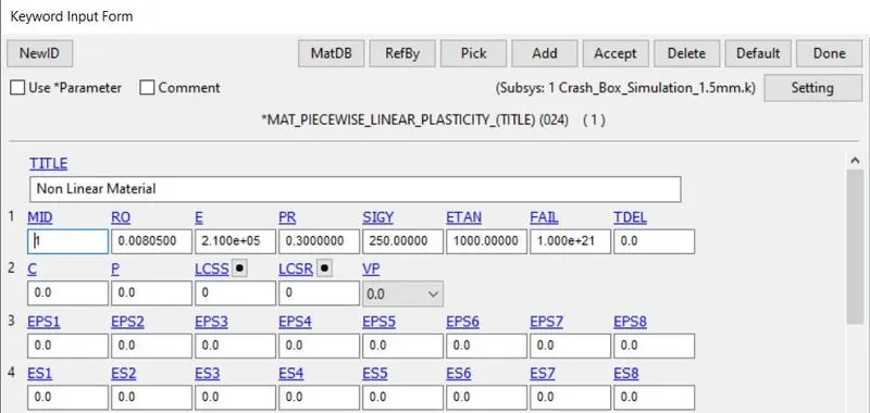
Thus the material card is ready as shown above.

Hourglass –

We will Define hourglass and bulk viscosity properties which are referenced using HGID in the *PART command. This keyword will control the hourglass energy which can be generated in the elements which produce no strain or stress.

• Go to Keyword Manager
• Select HOURGLASS Give it an hourglass ID and title.
• Select Hourglass control type (IHQ) as 2 and keep rest of the values as default.

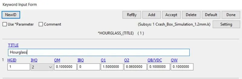
Now we will define these characteristics to the crash box part in PART keyword as shown below.

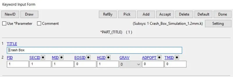
Contact –

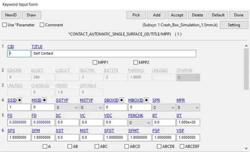
We will have to define self-contact for crash box as the crash box elements may have a contact between themselves after the deformation. So we will define AUTOMATIC_SINGLE_SURFACE contact with coefficient of friction 0.2 as shown below.

Control –

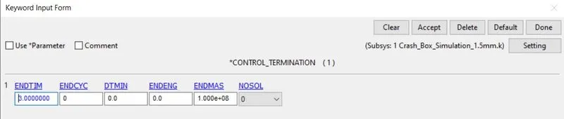
We will define the termination time of the simulation which is necessary to run the simulation. Thus we will define the termination time as 3 ms in CONTROL SIMULATION Keyword as shown below.

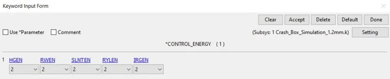
We will also define CONTROL_ENERGY card to provide controls for energy dissipation options as shown below.

Database –

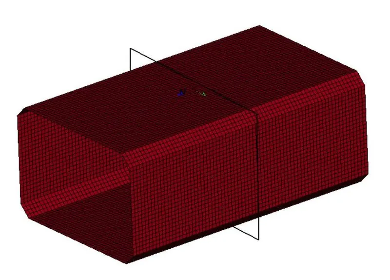
We have to find cross sectional forces generated in the middle of the crash box, as we will create a cross section at the middle.

Cross-Section –

• Go to Create Entity
• Under Database sub panel, select Cross Section and go to Cre to create a new cross-section.
• Select the node and the axis where the cross section plane must be located and then click on Apply. The cross-section will be created as follows.

History node –

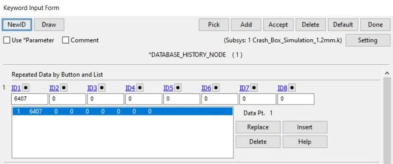
We will create a node history database card as we want the acceleration plot at a node in the middle potion of the crash box.

• Go to Keyword Manager
• Select DATABASE > HISTORY_NODE.
• Select node with ID 6401 in ID1 and click on Accept. Thus the node history database is created as shown below.

Binary Plot –

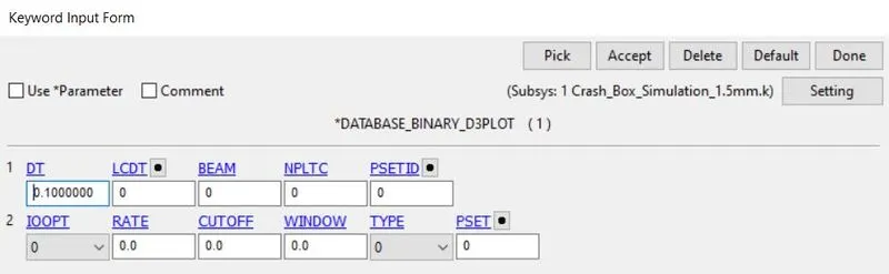
After defining all the conditions required for simulation, we can generate output requests or results which we are interested in the model. So we will define BINARY_D3PLOT under DATABASE keyword and specify Time interval between outputs DT as 0.1 ms.

In Database ASCII, we will ask for GLSTAT, MATSUM, NODOUT, RCFORC, RWFORC, SECFORC, SLEOUT, etc each with DT as 0.1 ms.

Now we will check our model with the Model Check command in Keyword Manager.

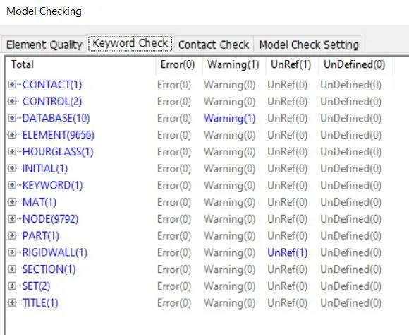
From the model Keyword check window, we can see that there are no errors and the warnings can be ignored.

After creating all the necessary files for simulation and checking the model, we will save the model as Keyword file with .K extension. To run the model, we will go to File > Run LS-DYNA. We will browse this keyword file and then run the simulation for shell thickness 1.2 mm and then for shell thickness 1.5 mm as shown below.

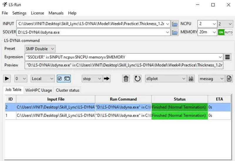
The simulation ended with Normal Termination so both the model was successfully simulated as seen above.

RESULTS AND PLOTS:

To run the simulation, we will open the binary d3plot file form specified path. Then we will click on Play button on Animation Toolbar. The resulting animation is shown below.

Results of 1.2 mm thickness Crashbox –

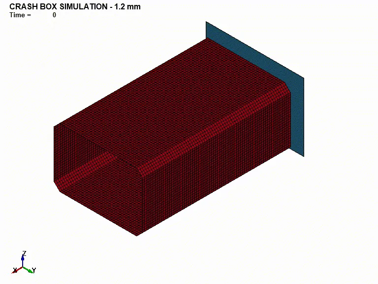
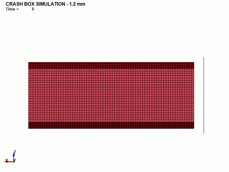
Based on the above simulation, we can see that the crashbox doesn’t deform after its impact on the rigidwall and bounces back. The kinetic energy of the crashbox is transferred to rigidwall or converted to internal energy, so after the impact the rebound velocity reduces. This is not the real case scenario and thus we may achieve some unrealistic plots as well.

Von-Misses Stress –

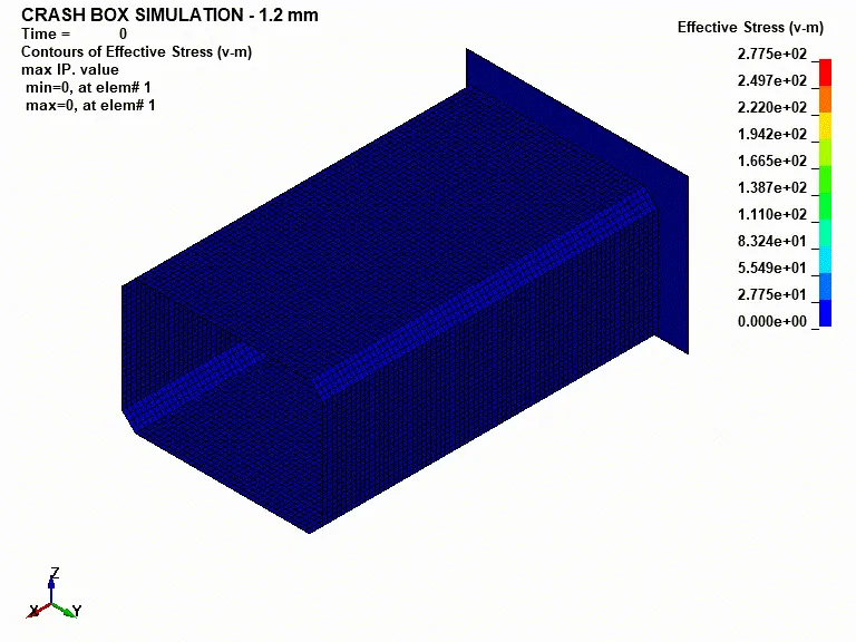
In the above animation, we can see that after the impact, there are stresses developed throughout the crashbox. Initially the maximum stress occurs at the region near the rigidwall. Then we can see stress fluctuation throughout the crash box. The stress distribution is uneven due to the vibrations induced in the crashbox after the impact. The maximum stress induced in the crashbox is 277.5 MPa.

Energies Plot –

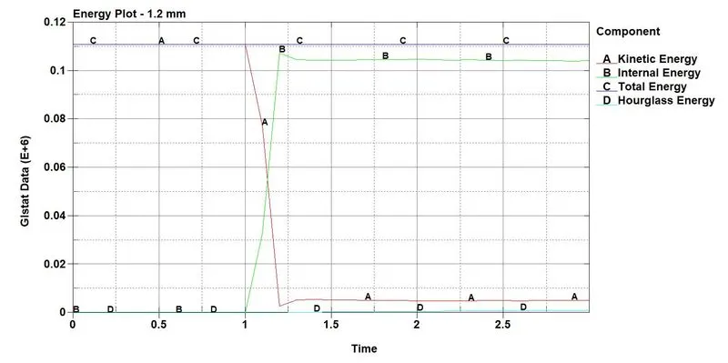
In the Energies plot, we can see that the kinetic energy of the model decreases after the impact at 1 ms and it gets converted to internal energy in the model. Thus the Total Energy of the system is constant. The hourglass energy generated in the model is almost negligible.

Cross-Section Force –

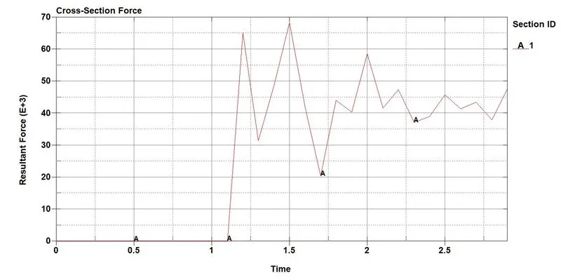
The plot of resultant force with time is along the length of the crash box where we located the cross-section plane. The maximum force of 68.5 kN is experienced at 1.5 ms after the impact.

Nodal Acceleration –

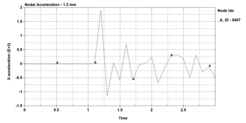
As the crash box is moving ad impacting in X-axis, we will plot the X-acceleration of Node 6407. The maximum value of the acceleration at Node ID 6407 is seen at 1.22 ms. After the impact, the crash box goes into vibration and thus we can see the acceleration plot positive as well as in negative X-axis.

X Stress –

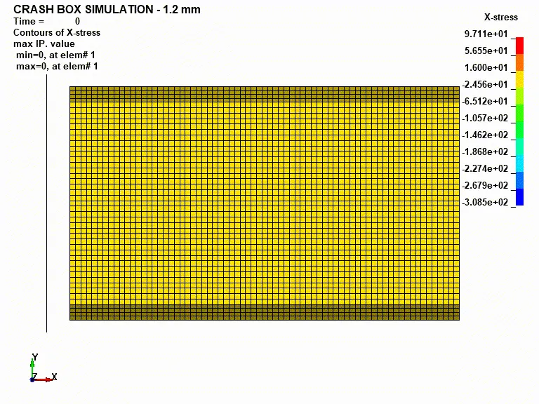
The stresses generated on crash box in X-axis are shown above. The maximum stress generated on X-axis is 97.11 MPa around the center region.

Y Stress –

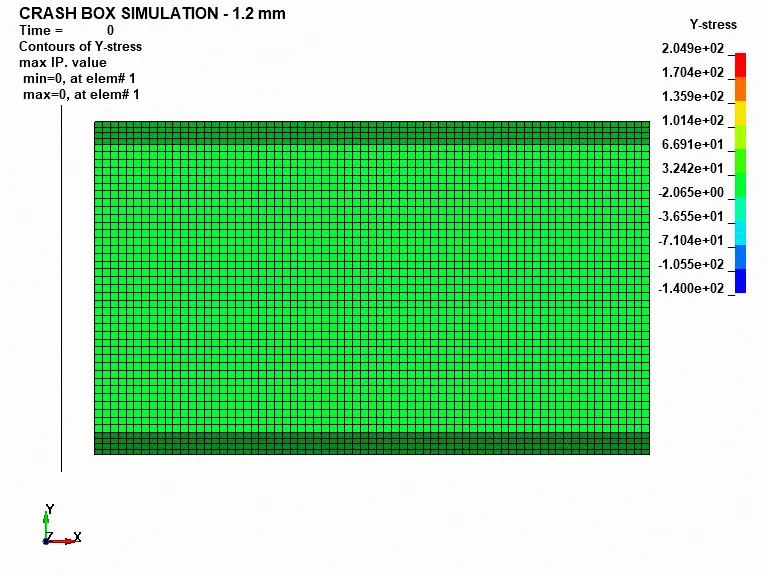
The stresses generated on crash box in X-axis are shown above. The maximum stress generated on X-axis is 204.9 MPa around the center region.

Effective Von-Misses Strain –

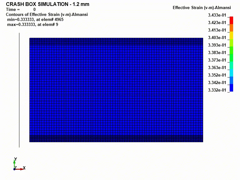
From the above shown Effective Von-Misses strain animation, we can see the maximum strain at the edge of the crashbox which is impacted to the rigidwall.

Results of 1.5 mm thickness Crashbox –

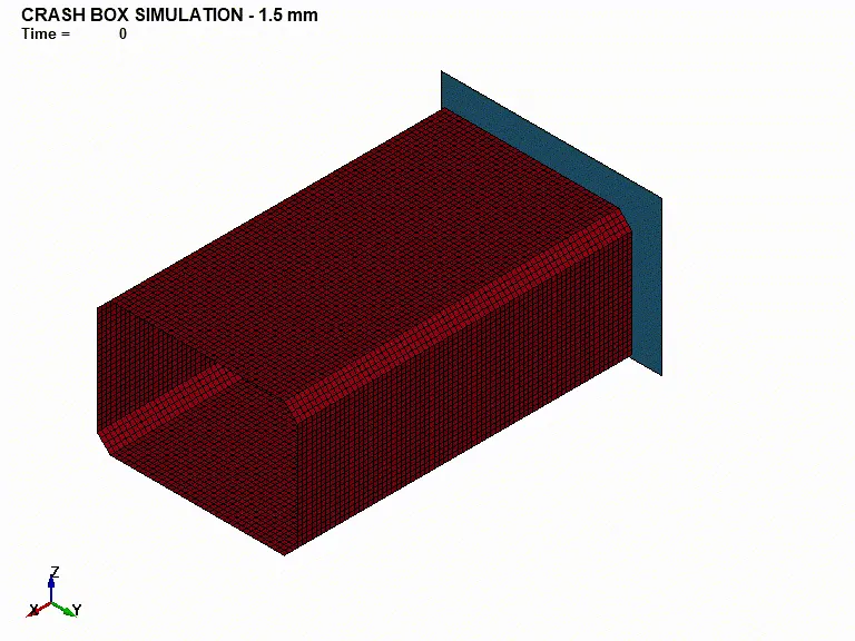
The animation of the crashbox with 1.5 mm thickness is almost similar to the crashbox with 1.2 mm thickness. The kinetic energy of the crashbox is transferred to rigidwall or converted to internal energy, so after the impact the rebound velocity reduces.

Von-Misses Stress –

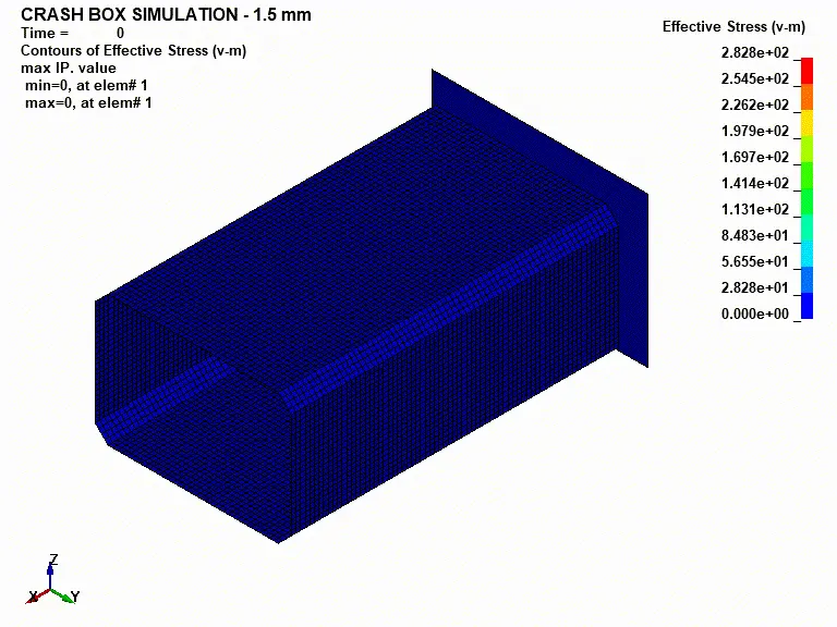
In the above animation, we can see that after the impact, there are stresses developed throughout the crashbox. Initially the maximum stress occurs at the region near the rigidwall. Then we can see stress fluctuation throughout the crash box. The stress distribution is uneven due to the vibrations induced in the crashbox after the impact. The maximum stress induced in the crashbox is 282.8 MPa.

Compared to 1.2 mm crashbox, the magnitude of stresses generated in this case is quite high. This is because the mass of the crash box increases with increase in thickness and thus increases the force which results in increased stress.

Energies Plot –

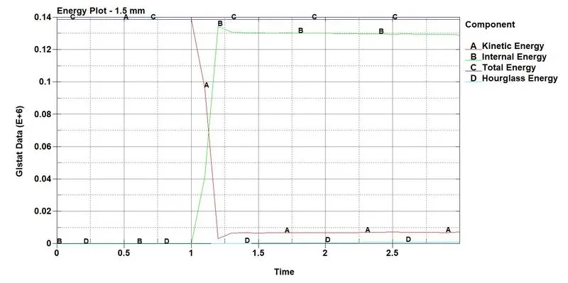
The nature of the energy plot is almost similar to the plot for 1.2 mm thickness. The difference being that the kinetic energy and total energy is more compared to the 1.2 mm thickness energy plot. As the thickness increases, the mass of the model increases and thus increases the kinetic energy which contributes in increase of total energy.

Cross-Section Force –

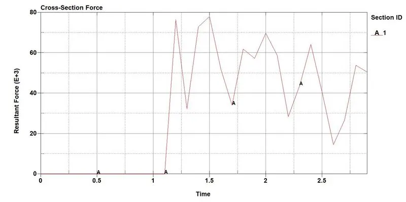
The plot of resultant force with time is along the length of the crash box where we located the cross-section plane. The maximum force of 78.5 kN is experienced at 1.5 ms after the impact. Comparing 1.2 mm thickness, we can see increase in the magnitude of force experienced at the cross-section as the mass is increased.

Nodal Acceleration –

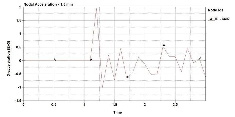
Comparing the acceleration plot with the plot for 1.2 mm thickness, we can see some negligible changes.

X Stress –

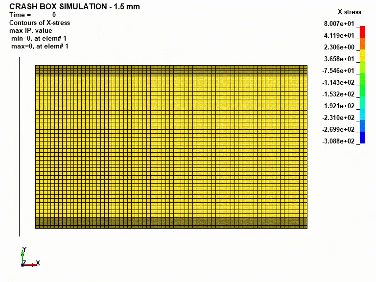
The maximum value of stress in X-axis is around 80.07 MPa. Comparing X-Stress plot for both the thickness values, we can see that the stress distribution is almost similar and due to the vibrations induced in the crashbox, it keeps on changing.

Y Stress –

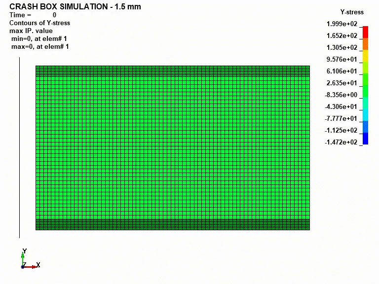
The maximum value of stress in Y-axis is around 199.9 MPa. Comparing Y-Stress plot for both the thickness values, we can see that the stress distribution is almost similar and due to the vibrations induced in the crashbox, it keeps on changing.

Effective Von-Misses Strain –

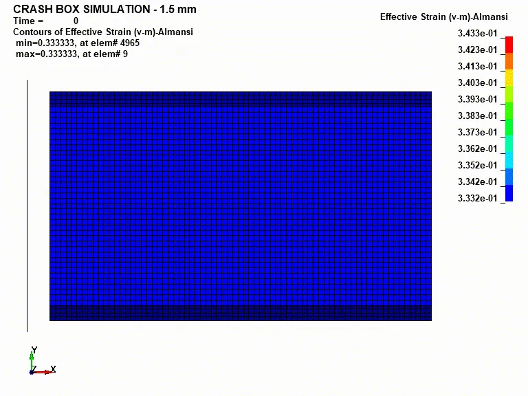
From the above shown Effective Von-Misses strain animation, we can see the maximum strain at the edge of the crashbox which is impacted to the rigidwall. This case is almost similar to the plot for 1.2 mm thickness.

CONCLUSION:

The impact of a Crashbox on a rigidwall was simulated in this project. By comparing all the results and simulation for two different thicknesses, we can say that there is some change in results and plots as discussed above. Thus, we can conclude that change in thickness of an object will change in the results and simulation behaviour of the model as the mass of the model or the mass matrix changes.