Crash Box Simulation using LS-DYNA
OBJECTIVE:
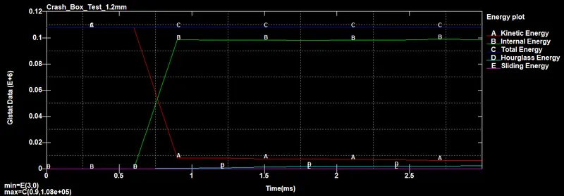
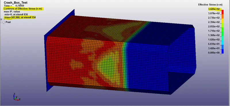
To create simulation results for a crash box under load and compare the plots for the obtained simulation results. The keywords are loaded to the model and saved in a new directory. The thickness of the box is changed and compared the results with the old thickness. Then the energy difference, stress, strain, von-mises for all the cases are plotted.
PROCEDURE:
There are three steps to be followed to achieve the simulation of the drop test, they are
Model setup,
Output requests,
Results.
MODEL SETUP:
The model setup is nothing but, the input model(keyword file) is studied and inputted with the suitable parameters in the LS-DYNA PREPOST deck, they are as follows
Title,
Assigning material cards,
Section creation,
Creating Rigidwall,
Contact interface,
Initial velocity,
Sectional_Force for nodes and elements,
Creating Control cards.
The model is opened through the command File--->open--->LS-DYNA Keyword file. or simply use the shortcut key ctrl+k. The unit system followed here is gm mm ms.
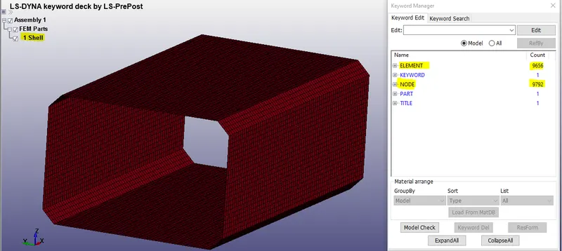
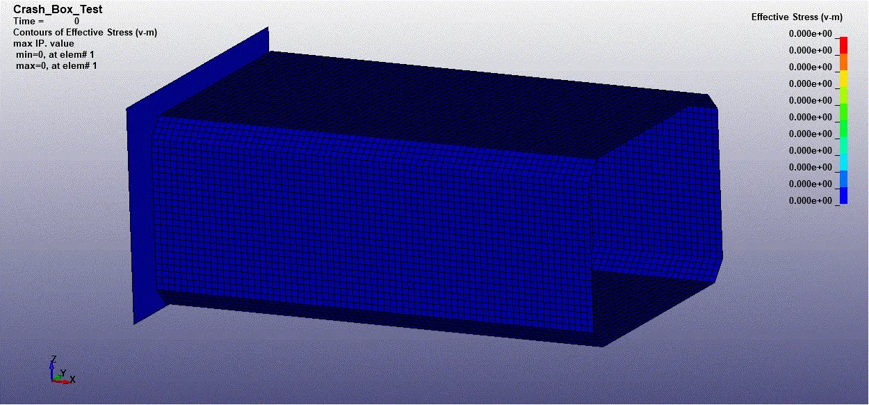
When the model is opened, it consists of only nodes and elements. The title of this test is saved as Crashbox Test.
Assigning Section card:
The material and the section for the shell are linked with the crash box through part creation. The command for the part is the Right-side toolbar--->model--->Keyword manager--->part command is used.
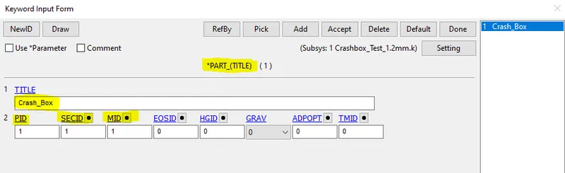
The section card is inserted through the command
Right-side toolbar--->model & part--->Keyword manager--->section--->shell. The thickness of the shell component is assigned as 1.2mm.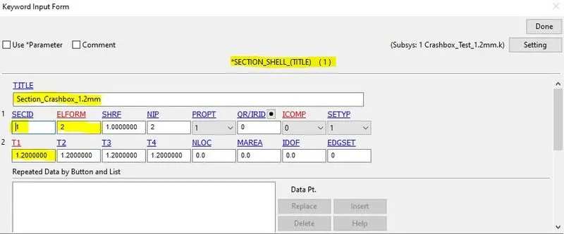
The other thickness of the shell component for the other case is assigned as 1.5mm.
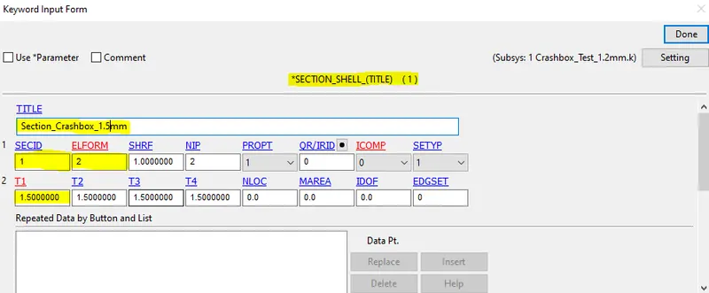
Then based on each case respectively the section is loaded to the input file.
Assigning Material card:
To assign the material to the parts separately, the command used is
Right-side toolbar>model>Keyword manager>Materials >24_piecewise_linear_plasticity card is used.
*Mat_024_Piece_Wise_Linear_Plasticity:
This is Material Type 24, which is an elastoplastic material with arbitrary stress as a function of strain curve and arbitrary strain rate dependency can be defined. Failure based on the plastic strain or a minimum time step size can be defined. The input values like density, young's modulus, Poisson's ratio, yield stress, and tangent modulus are inputted to the system.
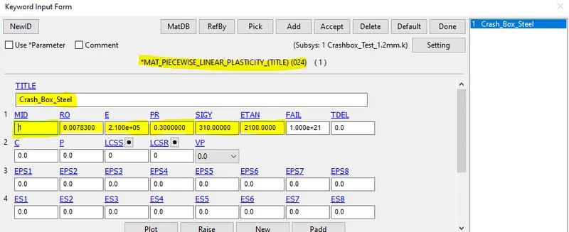
The material used for the crash box is steel and the mechanical properties of the steel is listed below,
- Density= 0.00783 `(gm)/(mm^3)`
- Young's modulus=2.10 e+05 `(gm)/(mm*ms^2)`
- Poissions ratio=0.33
- Yield strength =310 `(gm)/(mm*ms^2)`
- Tangent modulus = 2100 `(gm)/(mm*ms^2)`
The tangent modulus is taken as 1% of Young's modulus.
Rigid wall:
The next step is to create a Rigid wall in front of the crash box 10 mm away by using the *RIGIDWALL_PLANAR card
This is done by selecting Entity Creation > RigidWall > Create. The rigid wall type is selected as a Planar and defined vector with one point and a normal ie, 1n+NL here selected the one node, and the normal is created as a rigid wall. This rigid wall is translated/offset by 10mm from the crash box component.
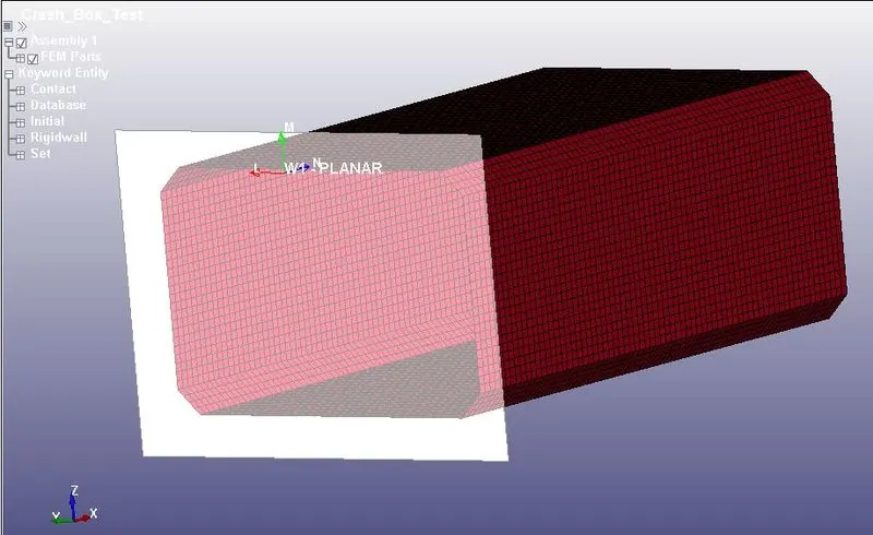
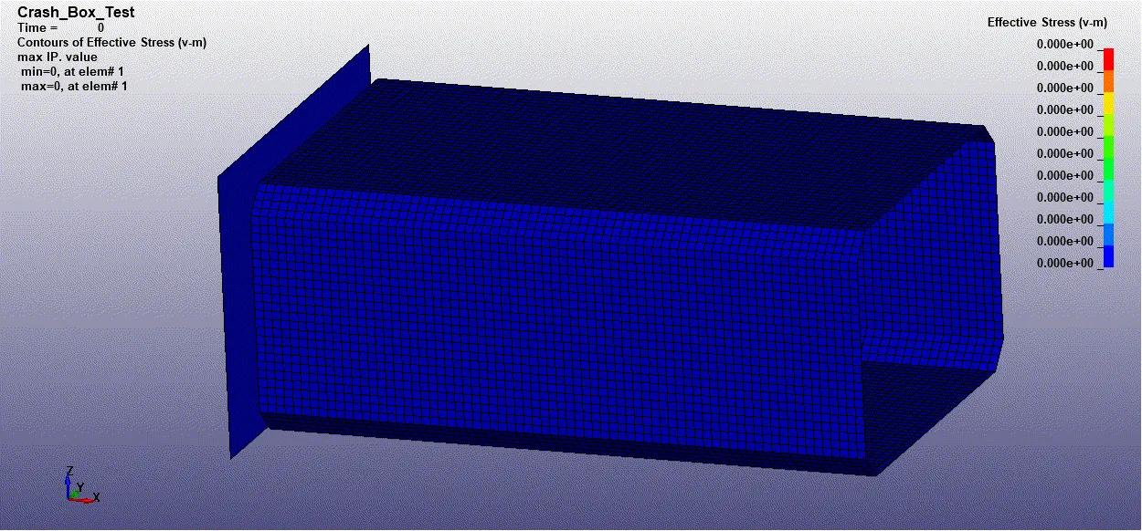
The white box in the window is a rigid wall and the normal is acting opposite to the global x-axis and it is
denoted in blue color.
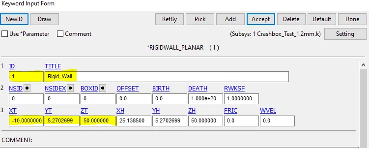
The rigid wall is placed correctly in the space where the x coordinates value is entered in a negative direction shows that the normal is acting in opposition to the crash box.
Contact Interface:
The objective of inputting the contact is to see how the nodes are reacting to external forces acting on the body. This gives us the exact solution to the problem. The surface-to-surface contact interface is used for the simulation. The command used for creating the contact interface
Right-side toolbar--->model--->Keyword manager--->Contact--->Automatic-surface to surface type is used.
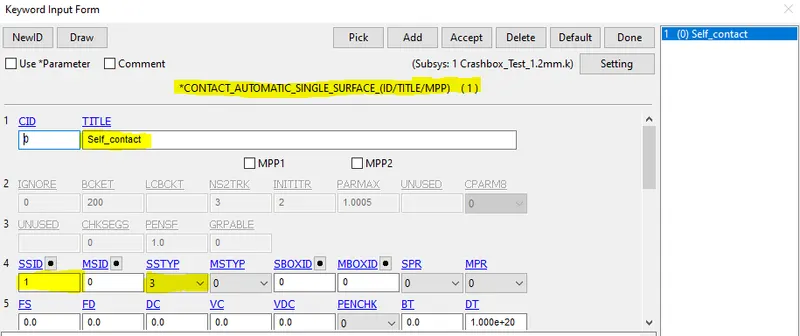
Create a Contact using
Model and Part--->Keyword Manager--->Contact--->Automatic Single Surface. The slave segment type (SSTYP) is defined by the Part ID, here there is no need to define a master surface so only the slave surface definition is sufficient.
After the automatic contact was created as the crash box elements are getting self contact during crashing ie, Automatic single surface here it was not needed to define the master surface because the crash box itself is master and slave.
Initial Velocity:
The next step is to define a velocity of 50kmph (13.8889 mm/ms) and assigned it to each node of the selected crash box component, under
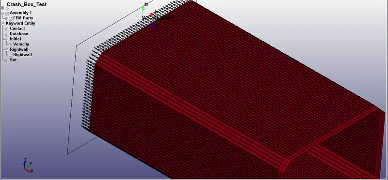
Right-side toolbar--->model--->Keyword manager--->Initial--->velocity command is used. The Crash box is selected by pick option with respect to part as shown below.
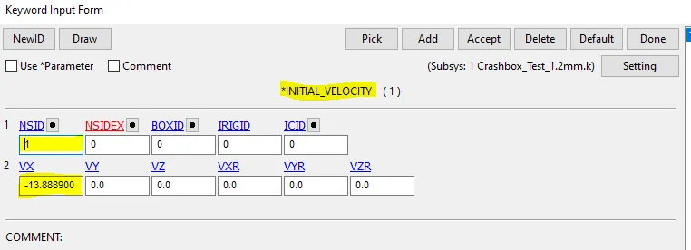
The initial velocity for the assembly is inserted in the x-axis tab in a negative direction shows that it is acting opposite to the global x-axis.
Sectional Force:
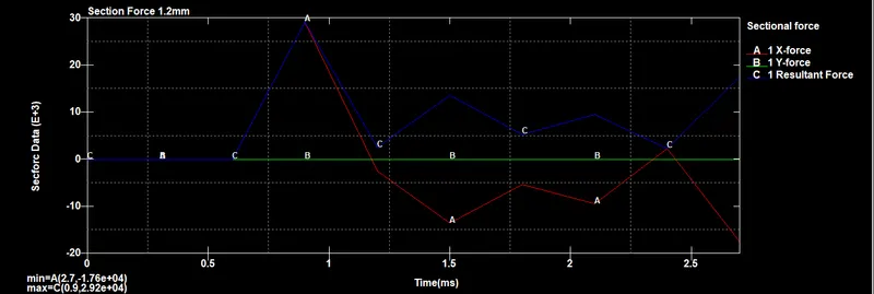
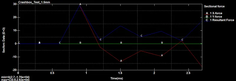
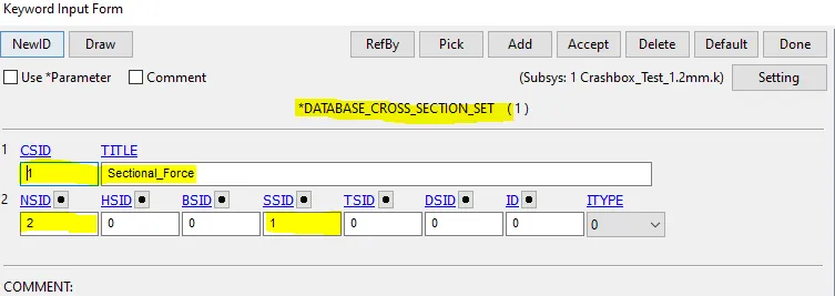
In the question, the sectional force for the nodes and elements at the centre of the crash tube along its length is to be recorded and plotted in LS-DYNA. To do that the command used here is
Model--->keyword manager--->database--->Cross_section_Set. command is used. The node set and the shell set is created using the command model--->create entity--->set_data--->set_node/elem. is used.
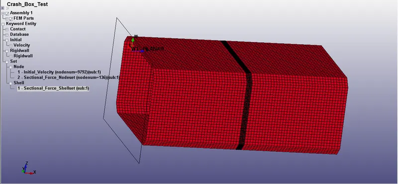
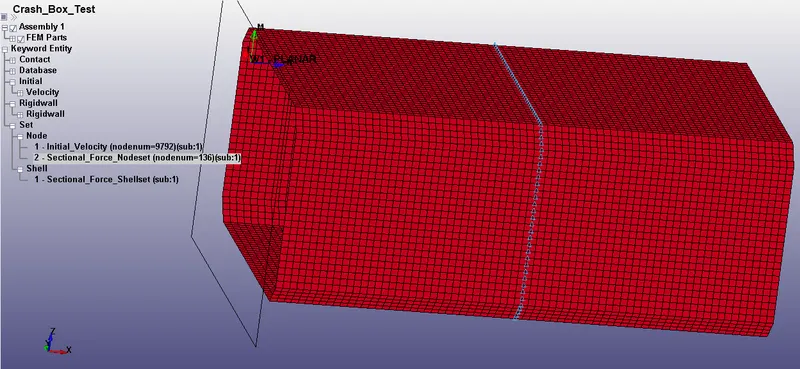
The approximate centre is considered and the nodes and elements are selected.
Control cards:
The control cards are used to get the output plots and simulation from the
Model--->keyword manager--->database--->ASCII/binary d3plot are used. The list of control cards for the output are listed below,
DATABASE_BINARY_D3PLOT --> Used to find out the animation of the process,
DATABASE_ASCII_NODOUT --> To find the Nodal motions,
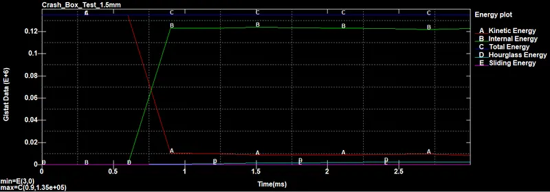
DATABASE_ASCII_GLSTAT --> To find the global statistics and energies,
DATABASE_ASCII_MATSUM --> To find the material energies,
DATABASE_ASCII_RCFORC --> To find the Resultant contact interface forces,
DATABASE_ASCII_SLEOUT --> To find the Contact interface energies,
DATABASE_ASCII_SECFORC --> To find the Cross-section forces data.
For generating section forces creating a specific node and element/shell list which defines the desired section of component is necessary. The selection of nodes and elements/shell lists is done by picking each node and element through Creating Entity--->Set Data--->*SET_NODE for node-set and
Creating Entity--->Set Data--->*SET_SHELL for element/shell-set.
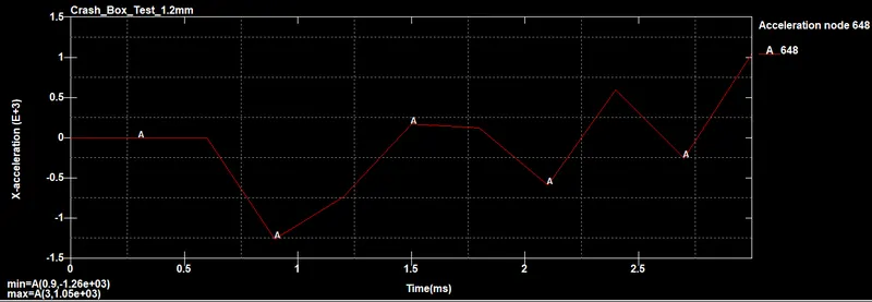
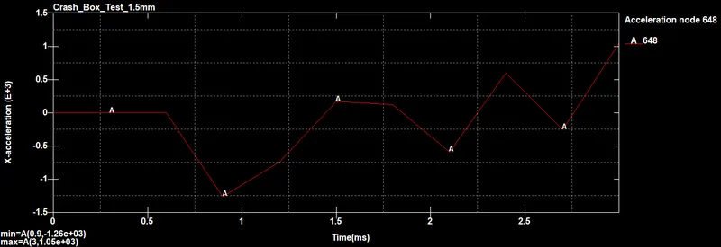
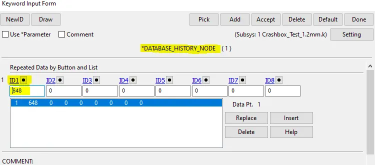
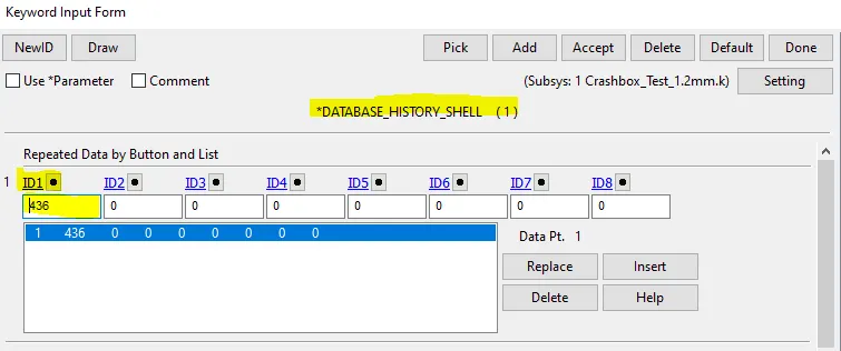
The acceleration plot of a node and element of the crash box can be done by picking the desired node and element by using *DATABASE_HISTORY_NODE and *DATABASE_HISTORY_SHELL card.
The termination time of the simulation is set to 3ms. It is set from the command
Model--->keyword manager--->control--->termination.
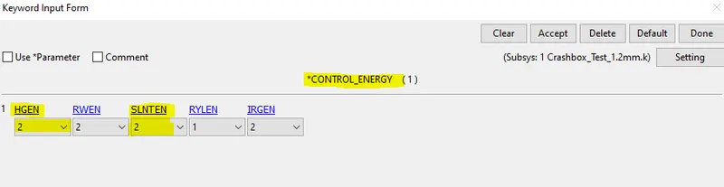
The Hourglass and the Sliding energy both are recorded and plotted using the command
Model--->keyword manager--->control--->energy.
Then finally the model is checked using the command Model--->keyword manager---> model check command is used.
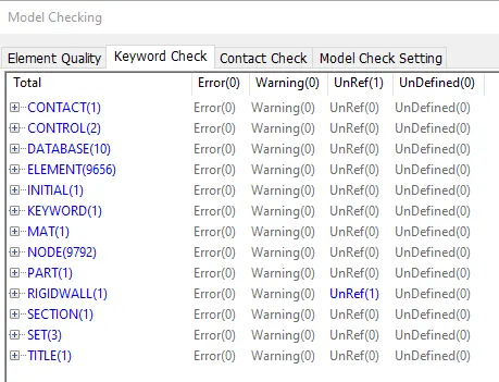
After assigning all the above-mentioned keywords, the model is ready for the simulation. The keyword file (.k) can be edited in notepad++ so that the comparison study can be done for the part which is having 1.2mm and 1.5mm thickness. Save the keyword for both files and opened in the LS-DYNA manager which solves the problem.
Output requests:
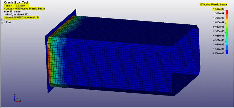
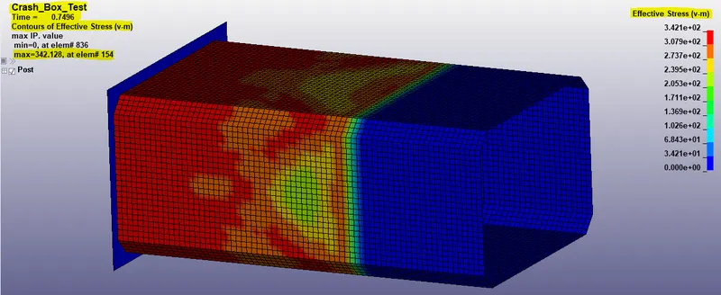
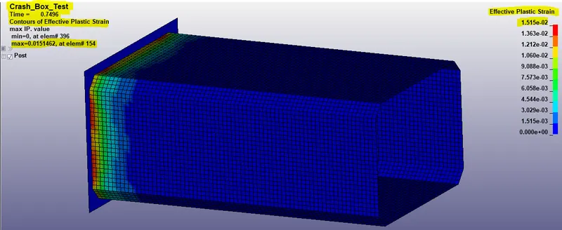
For the output request following files are loaded and displayed below through LS-DYNA.