Crash Box Simulation

Aim: The objective of this assignment is to run the simulation of a crash box crashing against a rigid wall, and plot graphs of stress, strain, forces, and displacement.

Requirement:

• The crash box should crash into a rigid wall created using the *RIGIDWALL_ keyword. Check the manual to understand and create a rigid wall.
• The material for the crash box is steel. The simulation needs to be started using elastic material to verify its correctness and later a nonlinear material card data will be provided. The thickness of the crash box is 1.2mm.
• The initial velocity for the crash box should be around 50 kmph
• The units system to be used is gm-mm-ms
• The simulation should satisfy either of the two situations - (1) It crashes on the rigid wall and rebounds completely or (2) it buckles and folds in the axial direction so as to come in self-contact.
• Once the simulation is completed and the results, as asked for below, are collected, run another simulation by increasing the thickness of the crash box from 1.2 to 1.5mm.

Procedure:

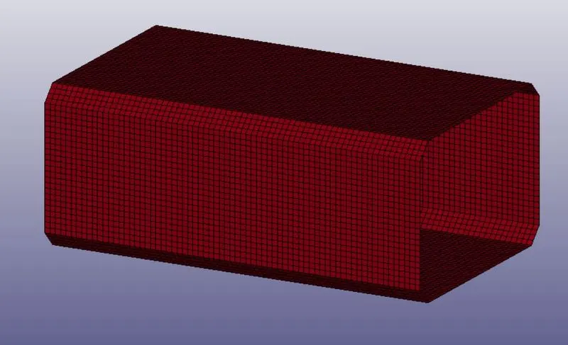
Step-1: Importing the .k file into the LS-PrePost interface

• Go to File < Open
• Browse for the provided input file
• Hit open

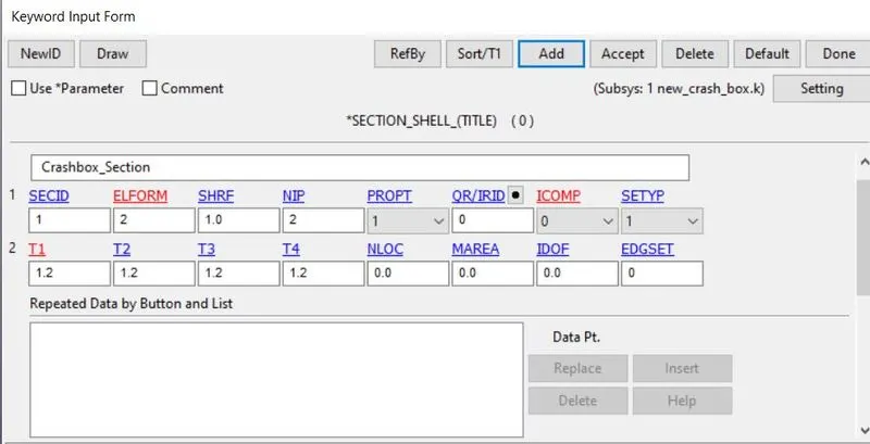
Step-2: Create a section card for the crash-box

• Go to Keyword manager< all< section< shell
• Put the information like the thickness of 1.2
• Keep everything else as default including element formulation and the number of integration points
• Hit accept and done.

Step-3: Creating a Material card

• Go to Keyword manager< all< material< Piecewise linear plasticity (024)
• Put information as given below
• Hit accept and done

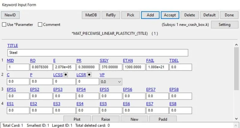
As we have to follow the unit system of g, mm, and ms we must put the following data in the material keyword

1. Density: 7.83*10^-3 g/mm3
2. Young’s modulus: 2.07*10^5 MPa
3. Poisson's ratio: 0.3
4. Yield strength: 370 MPa
5. Tangent modulus: 1.3*10^3

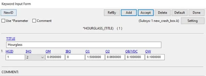
Step-4: Creating Hourglass card

• Go to keyword manager< all< hourglass
• Put hourglass control type as 2 that is viscous
• Hourglass coefficient as 0.05
• Hit accept and done

Note:

• Viscous versus Stiffness Control. Viscous hourglass control is recommended for problems deforming with high velocities. Stiffness control is often preferable for lower velocities, especially if the number of time steps is large. For solid elements, the exact volume integration provides some advantage for highly distorted elements.
• Automotive Crash Hourglass Control. For automotive crashes, the stiffness form of the hourglass control with a coefficient (QM) of 0.05 is preferred by many users.

Step-5: Assigning cards to the part

• Go to Keyword manager< model< part
• Select the part and rename it as crash box
• Assign section, Material, and Hourglass cards to that part
• Hit accept and done

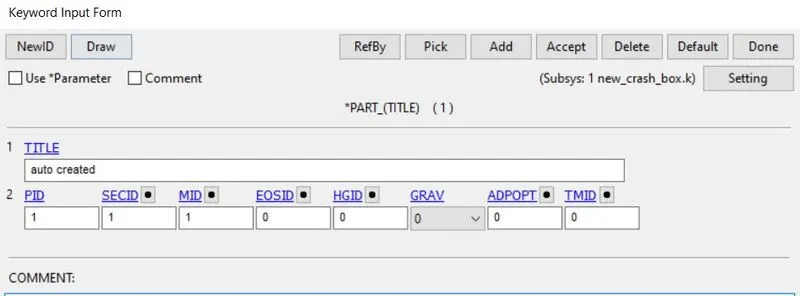
Step-6: Create a rigid wall

• Go to Entity creation< Ridigwall< Create
• Choose the Planer option, 1n+NL option, and click on the node where we want a rigid wall
• Move the rigid wall by 5/10mm to maintain some gap between the box and the wall by manipulating x-coordinates
• Hit apply

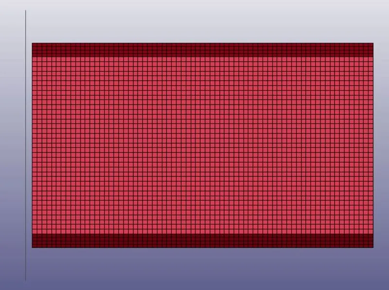
Note: We should ensure that the normal of the wall is facing the crash box and not in the same direction. In case our normal rigid wall and direction of travel of the crash box is the same, the box will penetrate the rigid wall and move ahead.

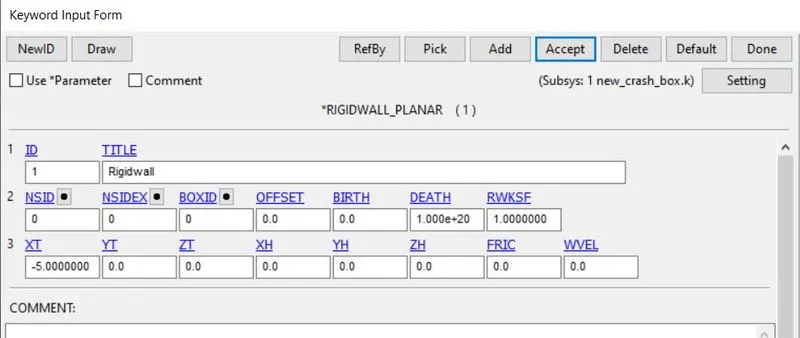
Step-7: Create Initial velocity

• Go to Entity creation< Initial< velocity< Create
• Choose by part and choose any node on the crash box to select all the nodes
• Put velocity value as 13.88mm/ms in an appropriate direction
• Hit apply

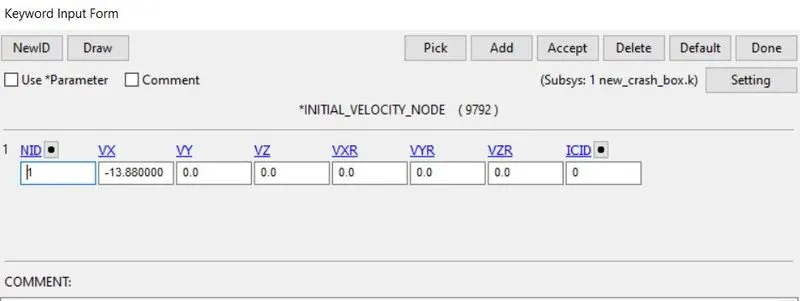
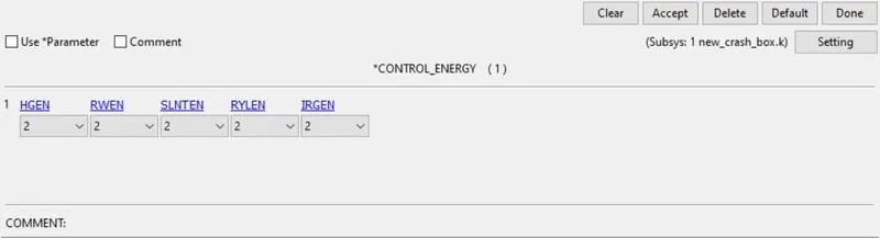
Step-8: Create a Control energy card

• Go to Keyword manager< all< control< energy
• Change all the options from 1 to 2
• Hit accept and done

Note: This card allows us to include hourglass energy in the energy balance. For example, if we keep HGEN as 1 then it will not compute hourglass energy. But, if we use HGEN as 2 then Hourglass energy is computed and included in the energy balance.

Step-9: Create a control termination card

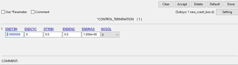
• Go to keyword manager< all< control< termination
• Put the End time value as 2ms. As the gap between the crash box is 10mm and the velocity is very high, the required results will not take much time.
• Hit accept and done.

Step-10: Create database cards

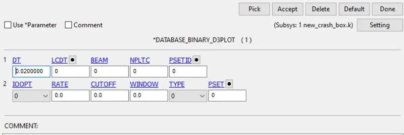
• Go to keyword manager< all< database< Binary D3plot
• Enter time as 0.02ms. Now the solver will write results every 0.02ms.
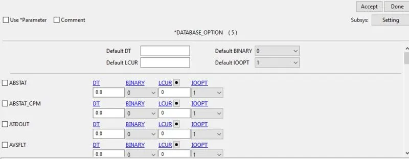
• Again, Go to keyword manager< all< database< ASCII
• Put default time as 0.02 and click on GlSTAT, RCFORC, RWFORC.
• Enter accept and do.

Step-11: Create a Database history card for the node

• Go to Keyword manager< all< database< History node
• Select the node that you want to retrieve results
• Hit insert, accept, and done.

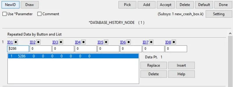
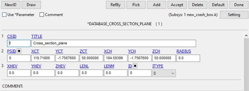
Step-12: Create a cross-section plane

• Go to entity creation< database< cross section
• Selection n1+NL option and select a node in between to create a section plane
• Hit apply

Step-13: Run the analysis

• Open LS-run
• Load the saved keyword
• Run the Simulation

Step-14: Check the results and plot the results

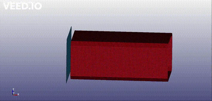
As expected, the crash box bounces back after crashing into the wall. Below is the gif showing the animation of the result.

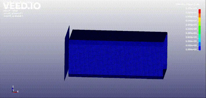
Von-Mises stress

Graphs:

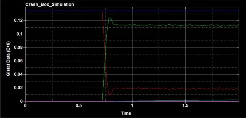
Energy Plot:

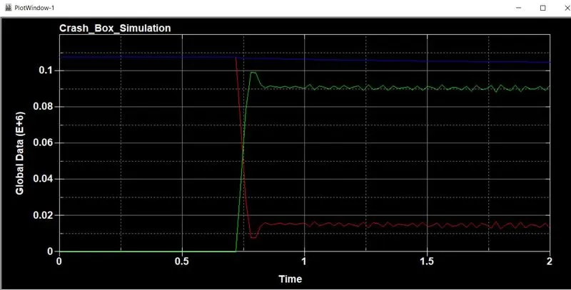
• Blue: Total energy
• Red: Kinetic energy
• Green: Internal energy

From the above plot, we can observe the following things:

• Kinetic energy starts from a non-zero value of 0.12Nmm and then drops around 0.7ms but did not reach zero during the entire simulation. We gave initial velocity which explains the initial kinetic energy in the body. Further, the box runs into the wall at around 0.7ms which reduces its velocity, and thus the kinetic energy drops. As the box bounced back after the crash and the simulation ended before it could come to halt, there is residual kinetic energy in the body.
• Internal energy starts from zero and increases after 0.7ms. As the body does not face any resistance initially, there are no internal resistive forces thus no stress in the body. However, at 0.7ms when the body hits the wall, the impact acts as an external load and the body resists this external load giving rise to internal energy.
• The total energy remains constant throughout the simulation

X-Displacement:

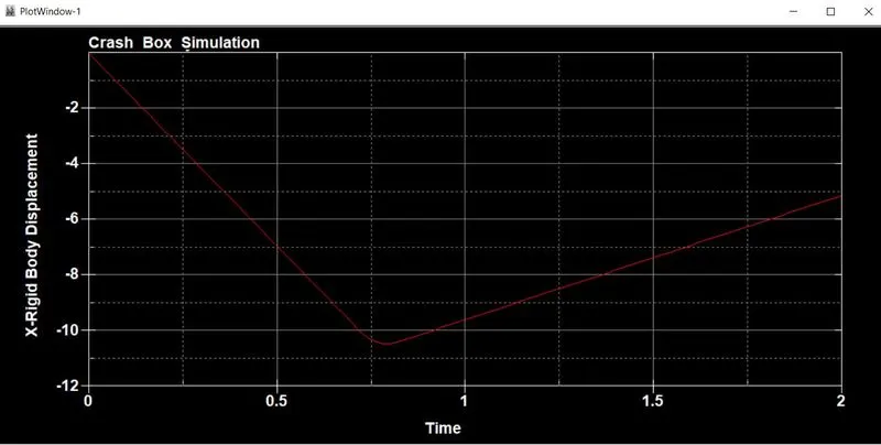
• As the body is given initial velocity in the negative x-direction, the displacement curve is negative.
• We can observe a drop in the curve which actually means that the body is moving forward till the collision
• We can also observe that the curve rises after the collision. This is because the body bounced back and traveled in the opposite direction
• If the direction of the initial velocity were in the positive x-direction, then the graphs would have increased first and then decreased after the collision.

X-velocity:

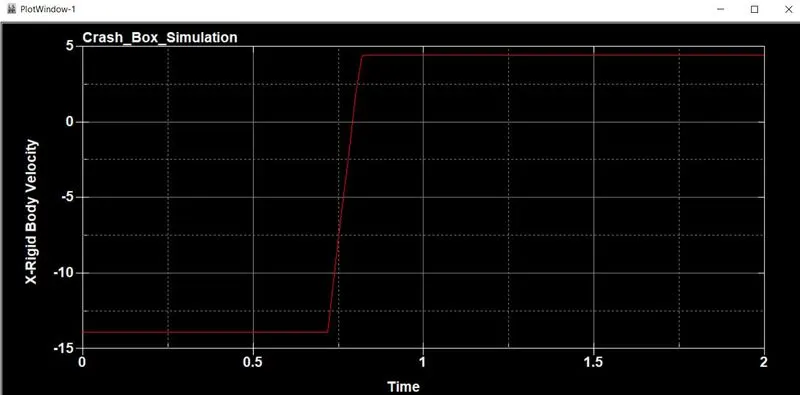
• As the body is given initial velocity in the negative x-direction, the velocity curve is constant and negative initially.
• After the collision, the curve increased, and then after a certain value, it became constant again. It actually shows the deceleration in the body
• If the velocity direction were positive, then the graphs would have dropped instead of rising which depicts actual deceleration.

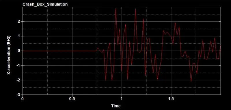
X-acceleration:

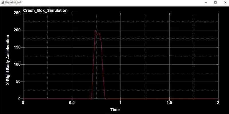
• There is no acceleration at the start and the end of the graph. This is because we have given a constant initial velocity and the body again bounces back with constant velocity.
• There is a peak and drop in the middle of the graph. This is because around that time-step, the body hit the wall which causes the change in velocity and thus gives rise to acceleration.

Rigid wall force:

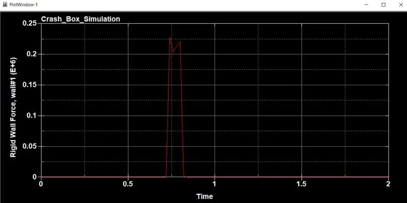
• There is no force at the start and the end of the graph. This is because there is no contact between the wall and the crash box at that time-steps.
• There is a rise and fall in the middle of the graph. This can be attributed to the fact that the box hit the wall at that time step and thus gave rise to forces.

GLSTAT (KE,IE,TE,and HgE):

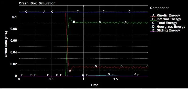
• We can observe minute fluctuations in the Hourglass energy.

X-acceleration of a node in the middle:

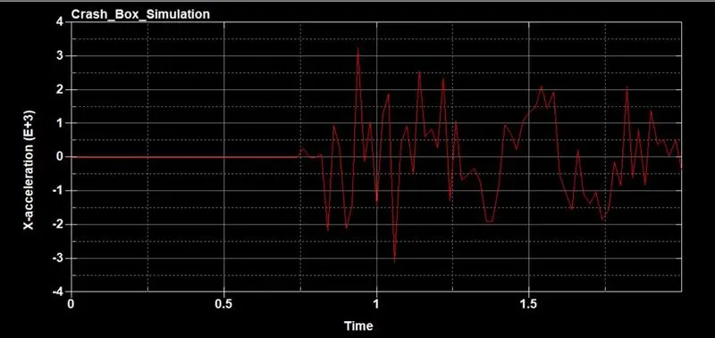
• As expected, it has zero acceleration till the box collides with the wall
• Post-collision, there are fluctuations in the graphs as the box bounces back. The impact travels from the element to element, and it reaches this node which explains this fluctuation.

Cross-section forces:

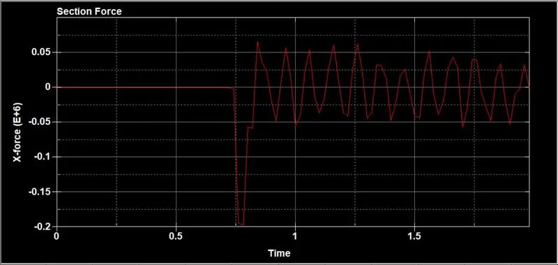
• There is no force in the chosen cross-section till the collision
• The graph for the force drops during the collision and then increases.

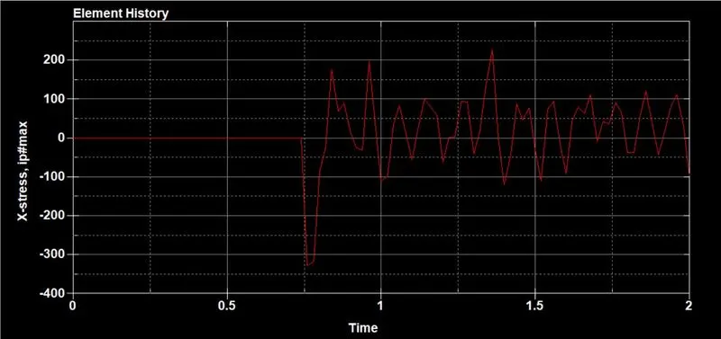
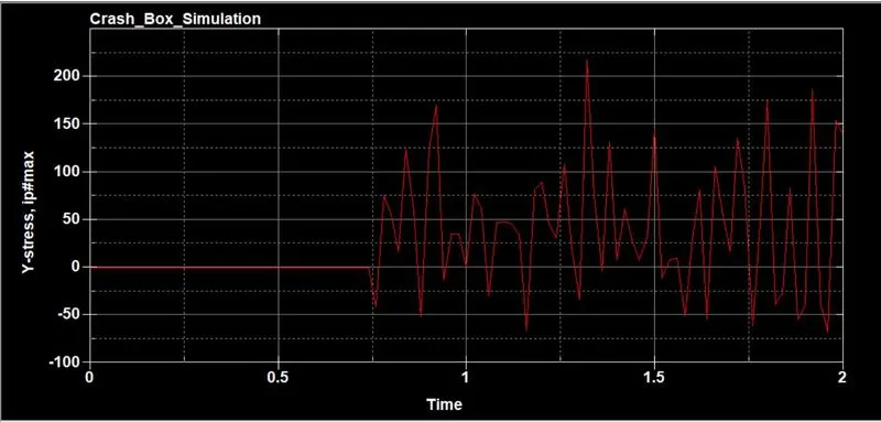
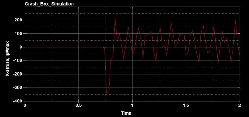
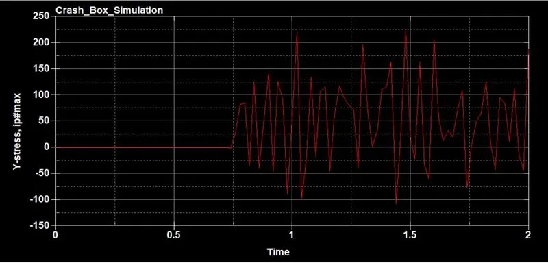
Stress in x,y, and z directions for 1.2mm crash box:

Plots for 1.5mm thickness crash-box:

Conclusion: Through this assignment, I have gained a better knowledge to use the software interface, preparing the model, and running simulations. Further, I have learned new keywords and their purpose.