Week 4 - CHT Analysis on Exhaust port

AIM: To perform Conjugate Heat Transfer flow simulation through a Exhaust port using Ansys Fluent

OBJECTIVE:

• • Give a brief description of why and where a CHT analysis is used.
  • Maintain the y+ value according to the turbulence model and justify the results.
  • Calculate the wall/surface heat transfer coefficient on the internal solid surface & show the velocity & temperature contours in appropriate areas.
  • How would you verify if the HTC predictions from the simulations are right? On what factors does the accuracy of the prediction depend on?

METHODOLOGY:

Introduction:

Conjugate Heat Transfer:

When multiple modes of heat transfer ie., variations of temperature within solids and fluids, due to thermal interaction between the solids and fluids are involved then the process is called Conjugate Heat Transfer. In solids, conduction dominates whereas in fluids, convection dominates. It is used in processes which involve variations of temperature within solids and fluids due to thermal interaction between the solids and fluids. Heat Transfer is the study of thermal energy exchange between the two physical bodies, the rate of tansferred heat is directly proportional to the temperature difference between the bodies. It is used in following engineering applications like heat exchangers, HVAC, and electronic component design.

Wall functions are useful in calculation the solutions near the wall. Y+ is a dimensionaless quantity that can be used to understand whether the mesh is coarse or fine which in turn determines the need for wall functions. The Turbulent flow have a smaller laminar region near the wall and if we are to resolve the gradients at such a small region, very small grid size is required.

Procedure:

1. Geometry preparation

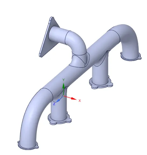
• IMPORT GEOMETRY IN SPACE CLAIM--> PREPARE --> VOLUME EXTRACTION --> Select edges
• 

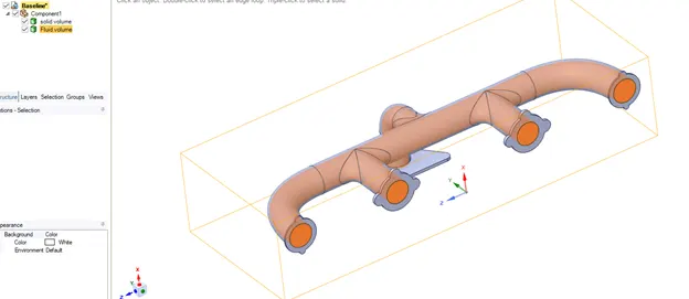
2. Mesh

• OPEN MESH -->ENTITY SELECTION > FACE SELECTION--> select the faces of the geometry to be mentioned as boundaries NAMELY INLET X,INLETY,OUTLET AND WALLS
• MESH -- > GENERATE MESH.
• Initailly keep the geometry in Y-direction. Now by using SECTION PLANE BUTTON, click and drag at the center to foam a line, so that it cuts the geometry.
• QUALITY --> MESH METRIC --> ELEMENT QUALITY --> C GRAPH ( AS LONG AS ELEMENT QUANTITY is not lower than 5%, SIMULAION RUNS)
• Add Basic size
• Add inflation for Y+ Value desired and first layer thickness calculated

• y + Calculation

  	PARAMETER	VALUE	Unit	Formulae
  Input
  	Free Velocity (U)	5.00000	m/s
  	density ( ρ)	1.22500	kg/m^3
  	Reference length (L)	0.17000	m	Inner diameter
  	Dynamic Viscosity (μ)	0.000018	kg/ms	Reference value from report
  	Reynolds number (Re)	58202.907		Re = ( ρ.U.L)/μ = >5*10^5 Turbulent
  	Kinematic Viscosity	0.00001		μ/ρ
  	skin friction coefficient, `C_f`	0.00509		`C_f = 0.079. Re^-0.25`
  	wall shear stress,`tau_w`	0.07788	m s ^2	`tau_w = 1/2. C_f.rho.U^2`
  	Friction velocity, U_f	0.252145062	m/s	`U_f = (tau_w/ρ)^0.5`
  	Turbulence model K - epsilon --> Y+ (>30)			Case 1
  	Y+	35
  	First layer thickness Delta y	0.002027178	m	Y+= (ρ.U_f.Deltay_1)/μ
  	First layer thickness Delta y	2.027	mm
  	Growth factor	1.8
  	No. of Layers	5
  	Total thickness `T_t `	21.28050103	mm	`T_t = Delta y *Gr^(n-1)`

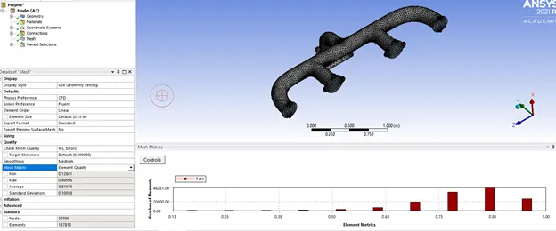
• Close the Mesh

3. Set Up

• DOUBLE CLICK SETUP -- > FLUENT LAUNCHER -->DOUBLE PRECISION.
• Ansys Fluent is opened.
• In Graphics window --> GEOMETRY AND CONSOLE window is displayed.
• SETTING UP DOMAIN -->MESH --> select CHECK. Then in CONSOLE WINDOW --> it shows 'CHECKING MESH…. DONE'
• To Change the Units, SETTING UP DOMAIN --> click Units
• SETTING UP PHYSICS --> SOLVER --> select Time = STEADY, Type = PRESSURE BASED & Velocity Formation = ABSOLUTE.
• SETTING UP PHYSICS --> MODELS > select ENERGY. VISCOUS MODEL --> Model --> K-epsilon Model, REALIZABLE K-epsilon Model, STANDARD WALL FUNCTIONS -->OK.

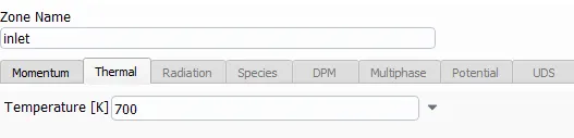
• SETTING UP PHYSICS-->BOUNDARIES -->ASK PAGE opens. Enter the values for Momentum, Thermal for both 'inlet' Then click OK.
• 
• 
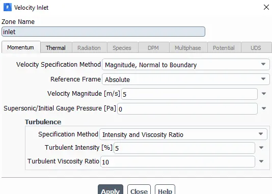
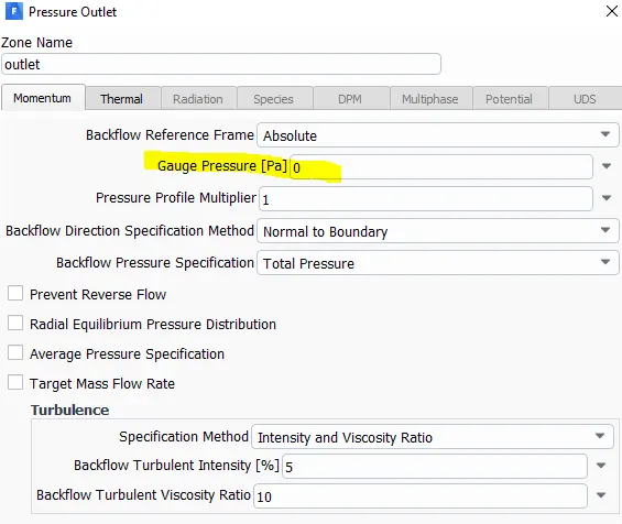
• FOR BOUNDARY 'outlet', the GUAGE PRESSURE (PASCAL) = 0 is available by default > Click OK.
• 
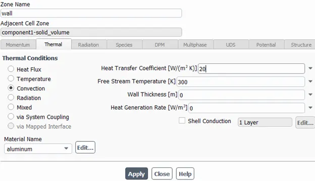
• Boundary wall --> Thermal convection heat transfer coefficient = 20
• 
• Solution MEthodology keep default

4. Solution

• SOLVING --> CONTROLS, REPORTS, INITIALIZATION, RUN CALCULATION.
• INITIALIZATION --> select METHOD = HYBRID --> click t=0 INITIALIZE
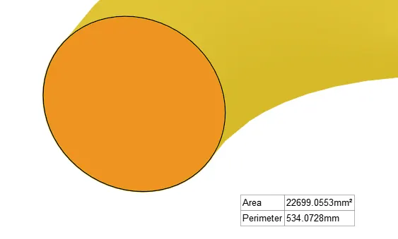
• Reference Value calcuation

Area	0.022699	m^2
Diameter	0.170003719	m

• RUN CALCULATION --> NO. OF ITERATIONS =500 and press CALCULATE.

5. Results and Discussion

CASE 1 Baseline

Residuals

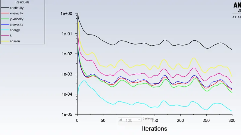
Inference: The solution can be considered as converged as variation of residuals are less and follows same pattern.

Velocity contour

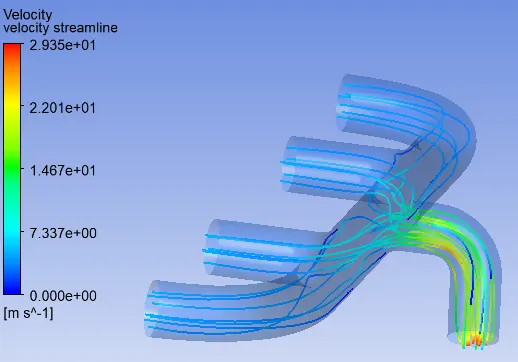
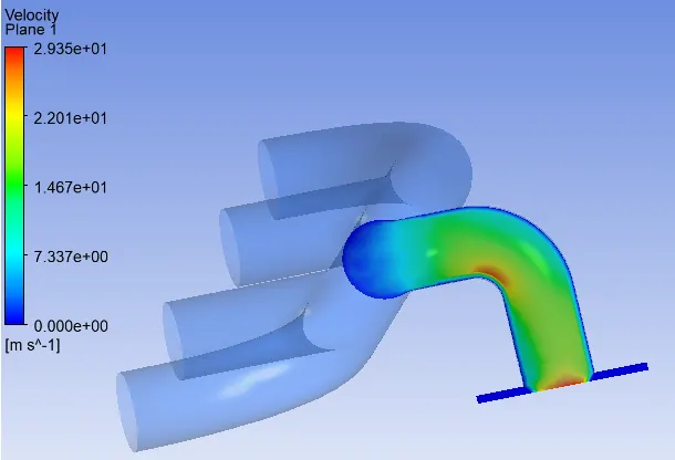
Inference: It is envisaged from the contour that at the region where all the exhaust gases merge has more less area in comparison to thier areas at induvidual inlet. As per the mass conservation theory the mass flow rate at the inlet and outlet remains the same. since Area decreases at the merging region it is compensated by increase in velocity to keep mass flow rate constant. Thus Velocity is high at that region which is explicitly seen in the stramline diagram. Max Velocity is 29.35m/s.

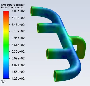
Temperature Contour

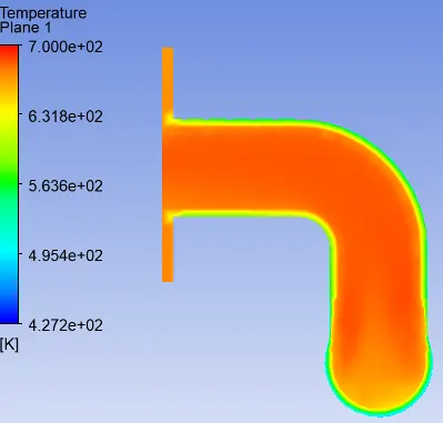
Heat transfer Coeffficient

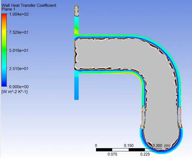
Inference: It is clear from the plot that at the region where exhaust gases merge the velocity is maximum or a high Reynolds number leads to a high heat transfer rate, therefore, higher heat transfer coefficients.

CASE 2 Inflation with suitable Y plus value w.r.t K epsilon model

2. Maintain the y+ value according to the turbulence model and justify the results?

• y + Calculation

  	PARAMETER	VALUE	Unit	Formulae
  Input
  	Free Velocity (U)	5.00000	m/s
  	density ( ρ)	1.22500	kg/m^3
  	Reference length (L)	0.17000	m	Inner diameter
  	Dynamic Viscosity (μ)	0.000018	kg/ms	Reference value from report
  	Reynolds number (Re)	58202.907		Re = ( ρ.U.L)/μ = >5*10^5 Turbulent
  	Kinematic Viscosity	0.00001		μ/ρ
  	skin friction coefficient, `C_f`	0.00509		`C_f = 0.079. Re^-0.25`
  	wall shear stress,`tau_w`	0.07788	m s ^2	`tau_w = 1/2. C_f.rho.U^2`
  	Friction velocity, U_f	0.252145062	m/s	`U_f = (tau_w/ρ)^0.5`
  	Turbulence model K - epsilon --> Y+ (>30)			Case 1
  	Y+	35
  	First layer thickness Delta y	0.002027178	m	Y+= (ρ.U_f.Deltay_1)/μ
  	First layer thickness Delta y	2.027	mm
  	Growth factor	1.8
  	No. of Layers	5
  	Total thickness `T_t `	21.28050103	mm	`T_t = Delta y *Gr^(n-1)`

Inference: K- epsilon model is used since the reynolds number is high 58202.907 paving path for Turbulent flow. The suitable y + range for the model is 30-300. Thus here the y+ desired value is 35. The first layer thickness is 2 mm approx. Reference length is taken from reference report of result section and sikin friction coefficient formulat is w.r.t to Internal flow through pipe. Creating an inflation layer with a proper Y+ value near the fluid wall face is imperative.

At Reynolds numbers between about 2000 and 4000 the flow is unstable as a result of the onset of turbulence. These flows are sometimes referred to as transitional flows. Turbulent flow. If the Reynolds number is greater than 3500, the flow is turbulent.

Residuals

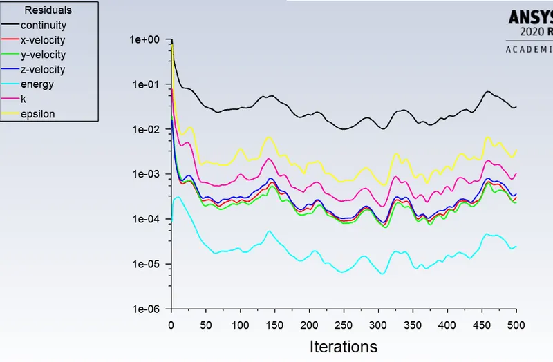
Inference: The solution can be considered as converged as variation of residuals are less.

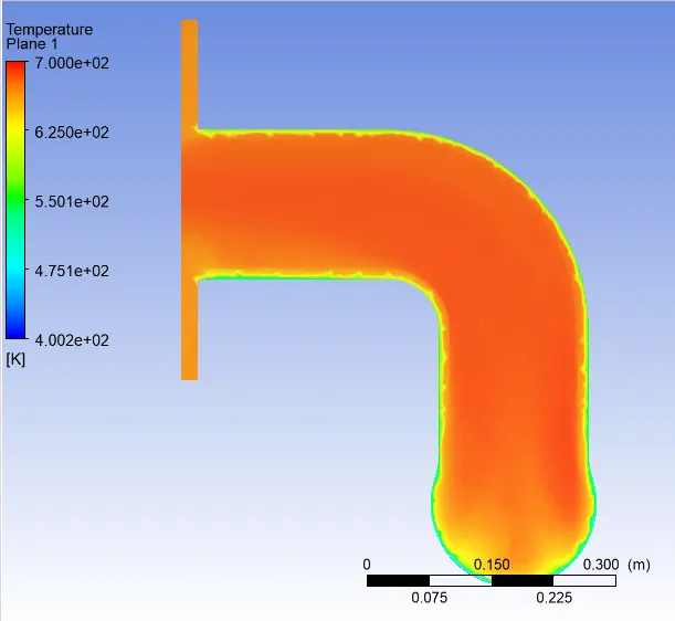
Temperature contour

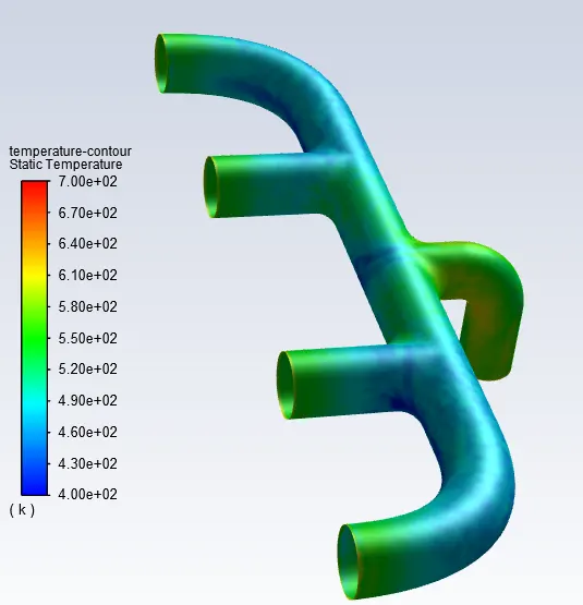
Velocity contour

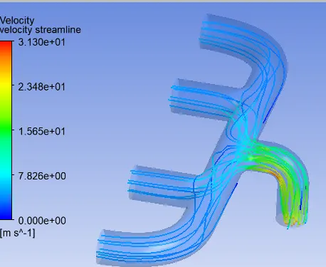
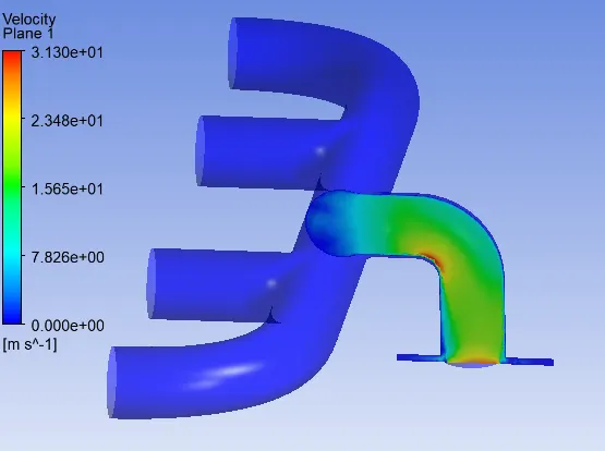
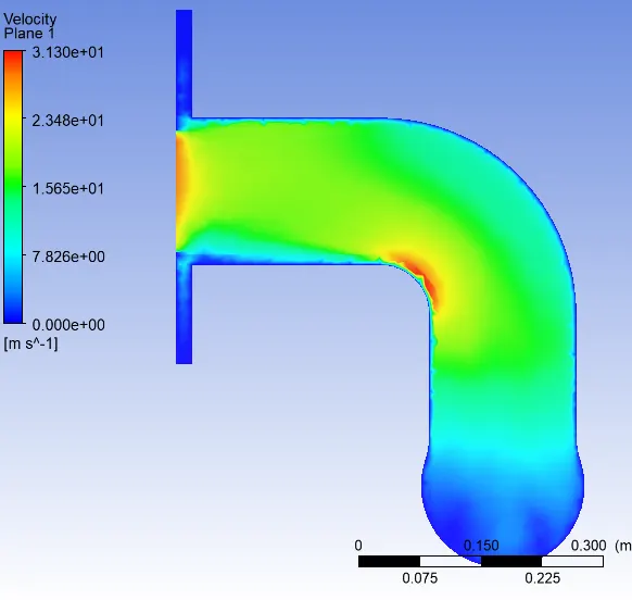
Inference: It is envisaged from the contour that at the region where all the exhaust gases merge has more less area in comparison to thier areas at induvidual inlet. As per the mass conservation theory the mass flow rate at the inlet and outlet remains the same. since Area decreases at the merging region it is compensated by increase in velocity to keep mass flow rate constant. Thus Velocity is high at that region which is explicitly seen in the stramline diagram. Max Velocity is 31.3m/s.

Heat transfer Coeffficient

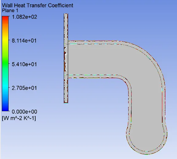
Inference: It is clear from the plot that at the region where exhaust gases merge the velocity is maximum or a high Reynolds number leads to a high heat transfer rate, therefore, higher heat transfer coefficients. Compared to baseline (Max Velocity is 29.35m/s.) the max velocity is higher in case 2 (Max Velocity is 31.3m/s) which in turn increases the heat transfer rate and heat transfer coefficient.

4. How would you verify if the HTC predictions from the simulations are right? On what factors does the accuracy of the prediction depend on?

Solution:

There are 2 ways by which the HTC predictions from the simulations can be validated/verfied

• Experimetal set up
• Analytical

Experimental set up : No research papers with complex shape like exhaust port has been set up and HTC were evaluated.

Analytical Approach: For simple shapes like flow over plate and internal flow through pipe we have analytical solution using the below emperical relation which relates the Nusselt number with respect to Reynolds number and Prandtl number or in other words Nusselt no. is the function of Reynolds no. and Prandtl no.

Based on Sieder Tate relation which correlates the Nu number with Re and Pr

`Nu=0.027 Re^0.8 Pr^(1/3)`

where:

• 	=	Prandtl number
  	=	momentum diffusivity
  	=	thermal diffusivity
  Cp	=	specific heat
  	=	Viscosity

Where,

Nu = h*L/K

L= Length of pipe

K=thermal conductivity are constant,

h = Heat Transfer Coefficient

Note that h increases as Nu increases and Nu increases as Re increases. By this procedure the 'h' can be found analytically.

4. CONCLUSION: The study of Conjugate Heat Tranfer through Exhaust port was simulated successfully.