CHT Analysis on Exhaust port
Conjugate Heat Transfer
The contemporary conjugate convective heat transfer model was developed after computers came into wide use in order to substitute the empirical relation of proportionality of heat flux to temperature difference with heat transfer coefficient which was the only tool in theoretical heat convection since the times of Newton. This model, based on a strictly mathematically stated problem, describes the heat transfer between a body and a fluid flowing over or inside it as a result of the interaction of two objects. The physical processes and solutions of the governing equations are considered separately for each object in two subdomains. Matching conditions for these solutions at the interface provide the distributions of temperature and heat flux along the body–flow interface, eliminating the need for a heat transfer coefficient. Moreover, it may be calculated using these data.
Applications
Starting from simple examples in the 1960s, the conjugate heat transfer methods have become a more powerful tool for modeling and investigating nature phenomena and engineering systems in different areas ranging from aerospce and nuclear reactors to thermal goods treatment and food processing, from complex procedures in medicine to atmosphere/ocean thermal interaction in meteorology, and from relatively simple units to multistage, nonlinear processes. A detailed review of more than 100 examples of conjugate modeling selected from a list of 200 early and modern publications shows that conjugate methods is now used extensively in a wide range of applications.
Boundary condition
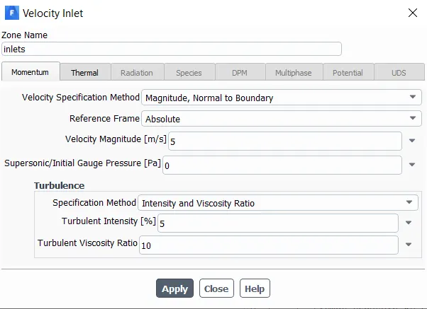
Inlet velocity = 5m/s
Inlet temperature = 700k
Pressure at outlet = 1atm
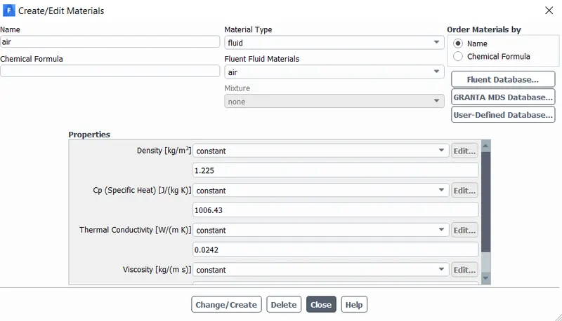
Fluid - air
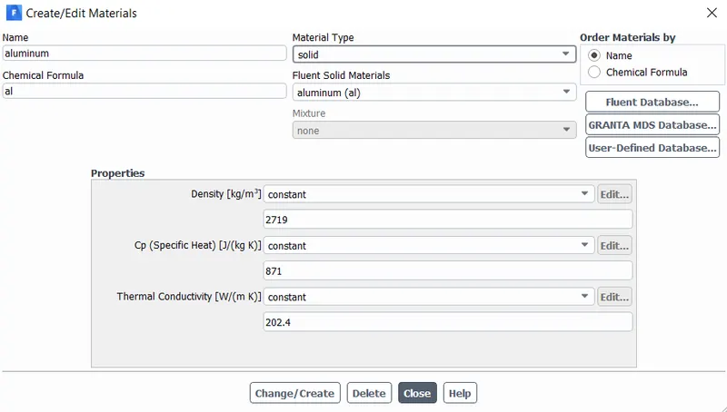
soild - aluminum
CHT analysis on the exhaust port
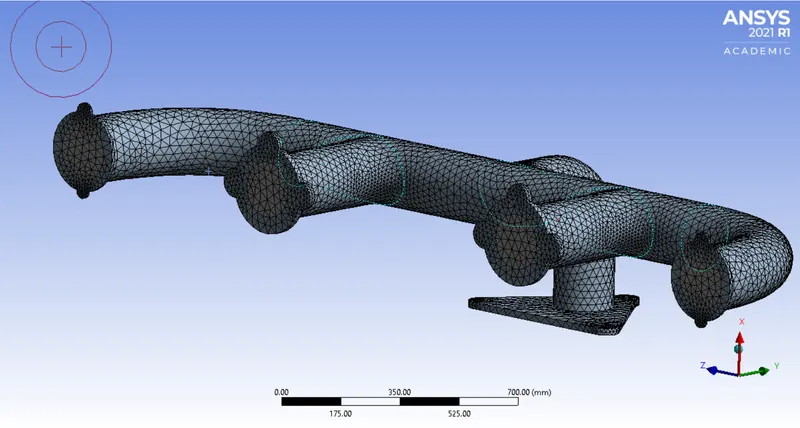
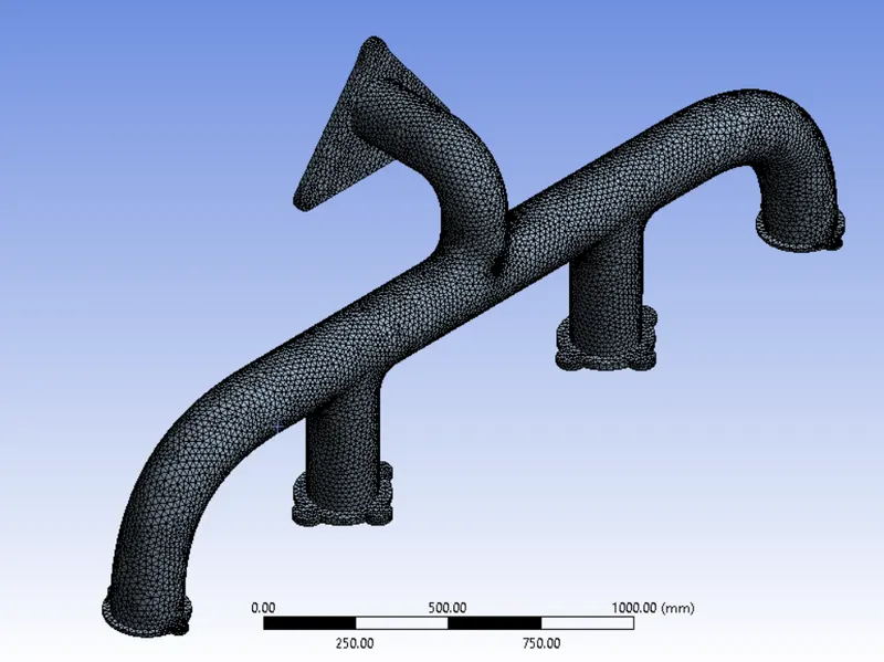
The figure represents the exhaust manifold of 4 cylinder engine
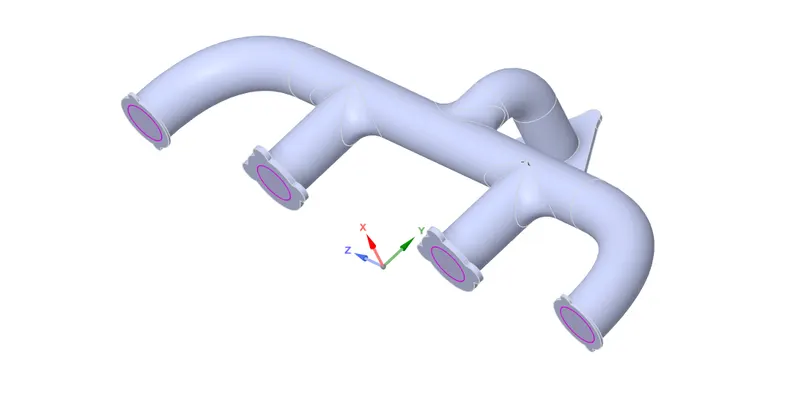
The geometry is prepared by using a volume extraction tool i.e, the fluid volume is extracted, the fluid and solid volume are shown in the figure
Fluid volume
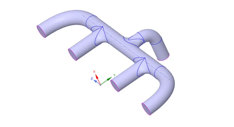
Solid volume
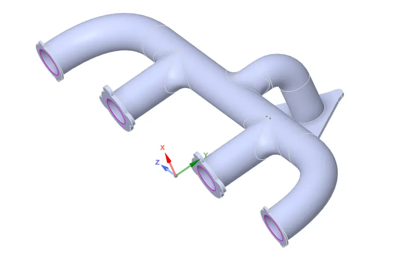
Now enable share topology in order to have conformal mesh between solid and fluid volume
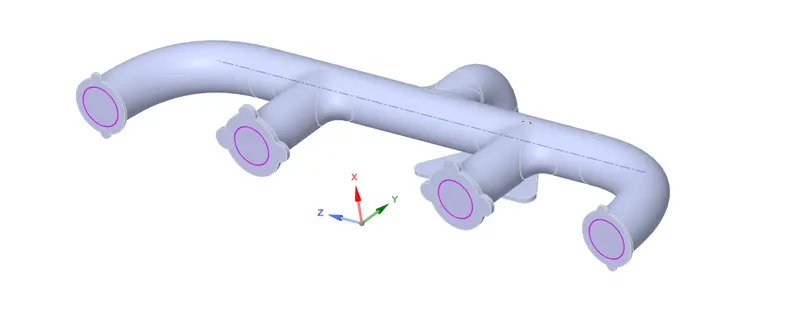
Case 1
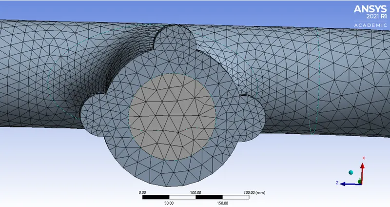
Baseline mesh with the element of 138035
Materials:
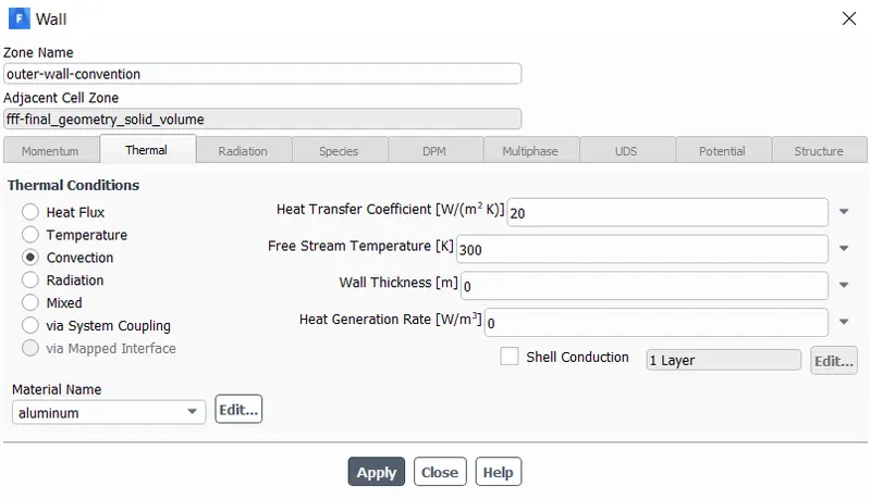
for solid aluminium is used and for fluid air is used
Inlet and wall condition
Post-processing:
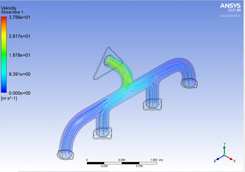
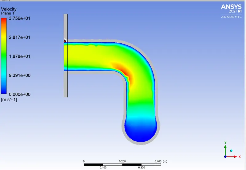
Velocity plot
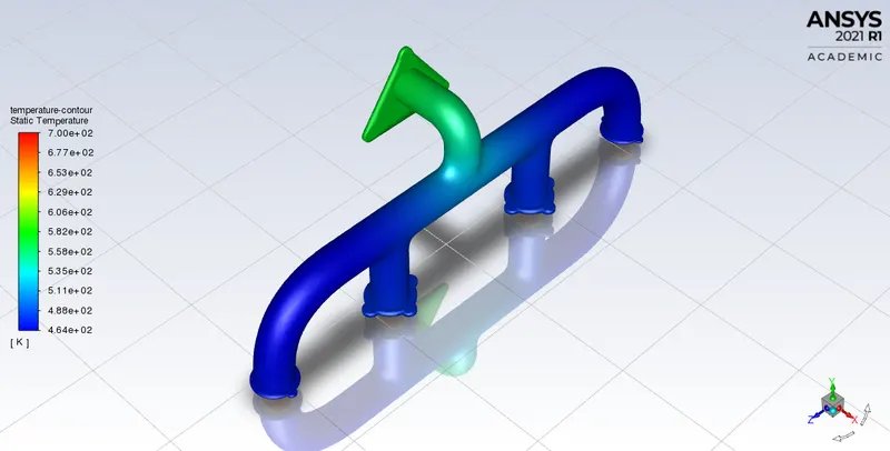
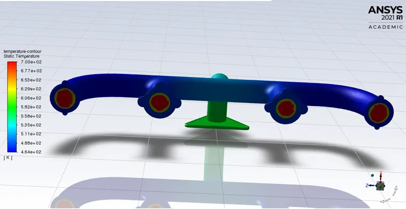
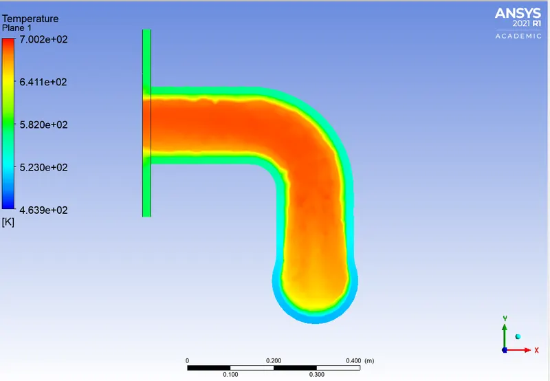
Temperature plot
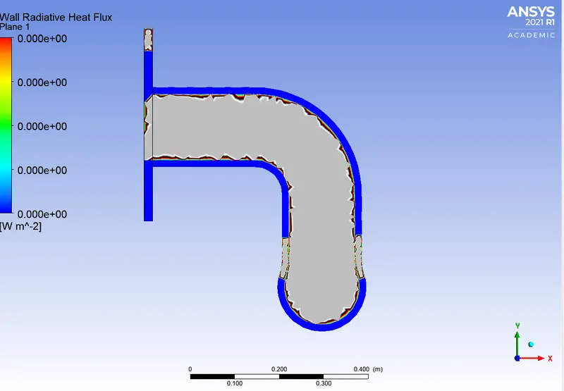
Wall radiative heat flux
Case 2
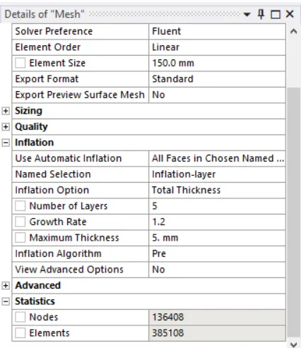
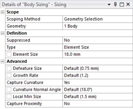
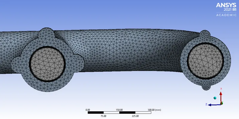
In this case, the mesh is made finer with an element size of 385108, and also 5 inflation layer is provided with a total thickness of 5mm
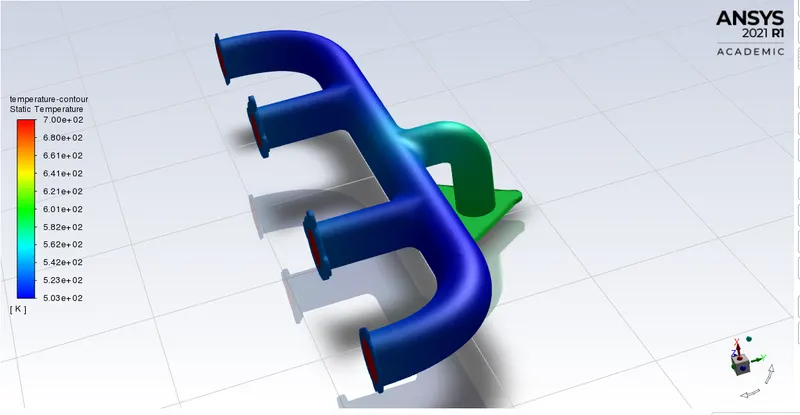
Temperature contour
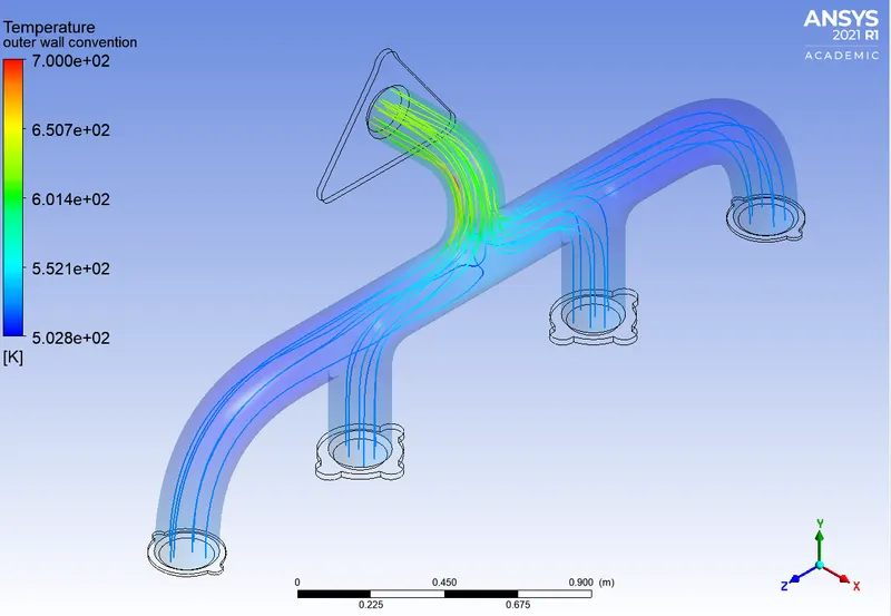
Velocity streamline
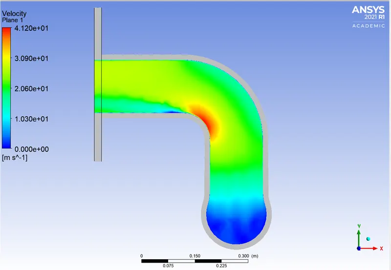
Velocity plot
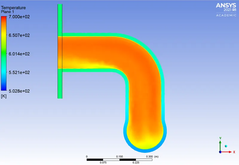
Temperature plot
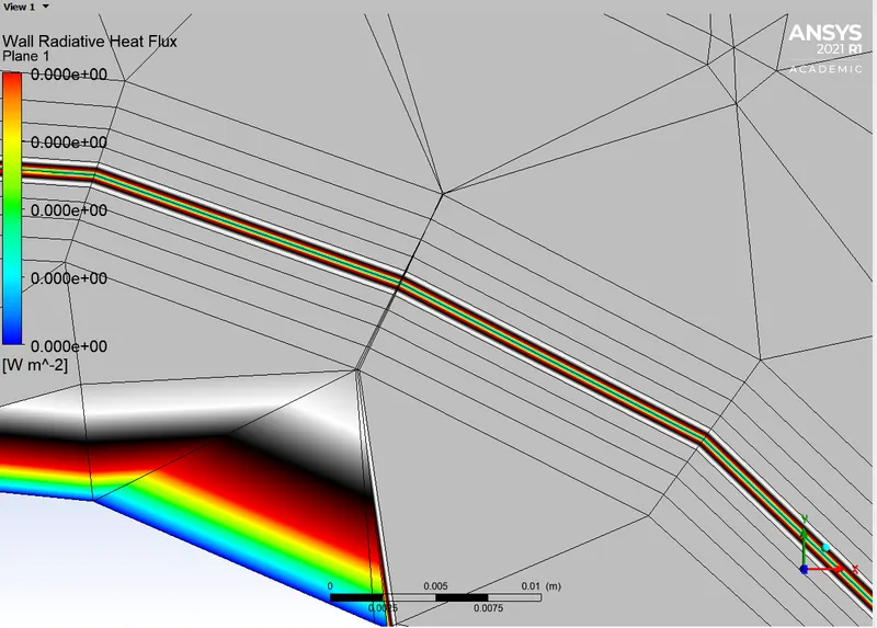
Wall radiative heat flux
Inference
InStreamline plots we can observe that the velocity at inlets is low compared to outlet, this is because of mas conservation. There are four inlets and only one outlet, all faces are same size i.e the area is same, and area times velocity is flow rate.
A1V1+A2V2+A3V3+A4V4=A5V5
where A1, A2, A3 and A4 are areas of inlets 1, 2, 3 & 4 respectively and A5 is area of inlets
V1, V2, V3 and V4 are velocities at inlets and V5 is velocity at outlet
here all areas are same so,
V1+V2+V3+V4=V5, and hence velocity at inlet is higher.
When we refined our mesh there was an increase in the values of wall heat transfer coefficient and velocity, so we can say that as the mesh gets more refined the results generated are more accurate.
Verification of HTC and factors affrcting it
Verification can be done in two ways
Physical experiment
Analytical method
Analytical method is done by Nusselt number
Nu=0.023*(Re^(0.8))*Pr^n
where,
Nu- Nusselt number
Re- Reynold's number
Pr- Prandit number (ratio of momentum diffusivity to thermal diffusivity)
After calculating the Nu number HTC can be computed using
Nu=hD/k
h- wall heat transfer cofficient
by this one can verify their predicted results
Factors affecting HTC
Element size
Mesh quality and mesh refinment
Inflation layers
Mesh at solid and fluid interface (it should be conformal mesh)