Week 4 - CHT Analysis on Exhaust port
Objective:
To simulate the Exhaust manifold in Ansys fluent for analyzing the heat transfer and the flow of fluid inside.
Conjugate heat transfer:
The term Conjugate heat transfer is used to describe that when there is a heat transfer between solid to fluid and vice versa.
The conjugate heat transfer (CHT) analysis is an iterative way to simulate the heat transfer between solid and liquid surfaces.
Applications of CHT:
Heat exchanger, cooling fins with natural or forced convection, etc. . . .
K Omega model:
More accurate for near-wall interactions than k-epsilon models. Ability to predict flow separation and accurate prediction for internal flow, curvatures.
Needs small inflation layer which increases the total cell count.
For this model, Y+ should be below 10 (Y+<10).
Using Matlab code total thickness is calculated with a desirable y+ of 3.
clear all
close all
clc

u = 5; %m/s
L = 0.15; %m
rho = 1.225; %kg/m3
mu = 0.000018375; %kg/m.s
Y_plus = input('enter desired value of Y+: ');

Re = u*L*rho/mu; %reynolds number

cf = 0.026/(Re^(1/7)); %skin friction coefficient

T_wall = 0.5*cf*rho*u^2; %wall shear stress

U_fri = sqrt(T_wall/rho); %friction velocity

del_s = Y_plus*mu/(U_fri*rho);

growthrate = 1.2; %growth rate of next cell from previous cell
no_layer = 6; % no of cells
tot_thick = del_s*2*1.2^(no_layer-1);

fprintf('\n Reynolds number is %d \n \n',Re);
fprintf(' first wall thickness is %d in m\n \n',del_s);
fprintf(' Total thickness of the cell %d in m\n', tot_thick);
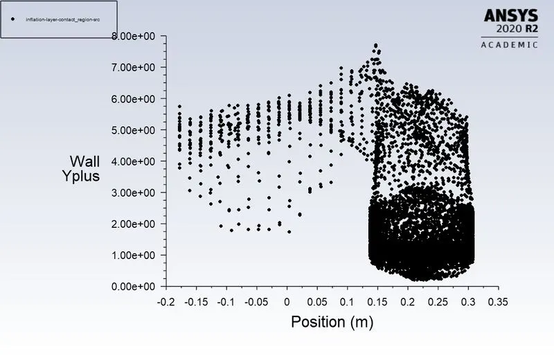
from the above chart, we can say that the y+ value is within 10. so we can use the K-omega model.
Meshing:
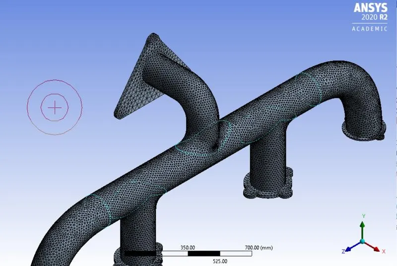
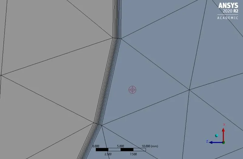
inflation layer:
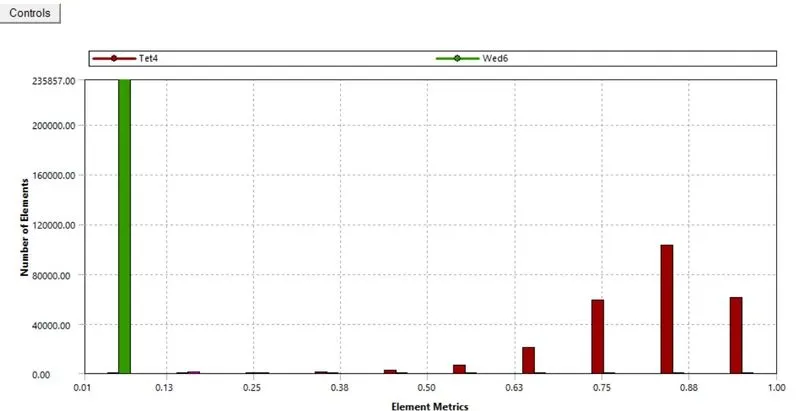
Element Quality:
Residuals:
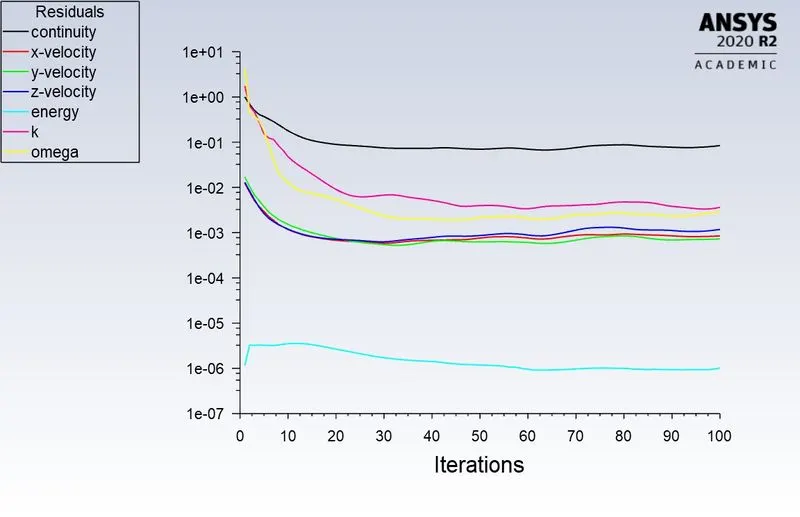
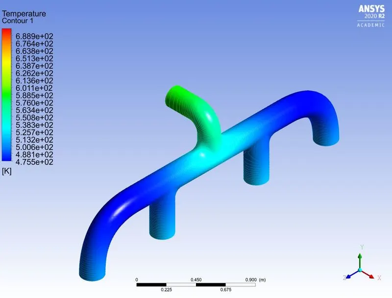
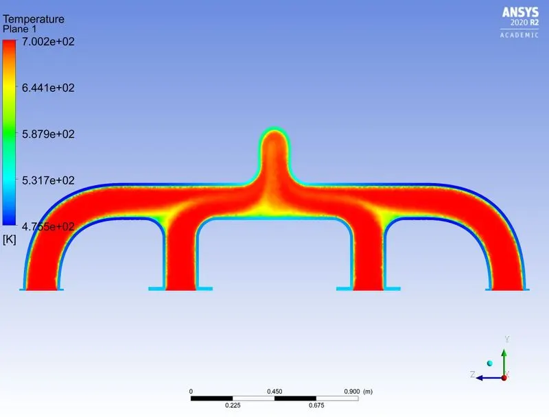
Since there is not much change in residual values and temperature variation in the temperature contour, thus the solution is converged.
Post-processing:
Temperature contour:
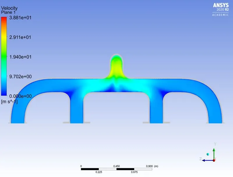
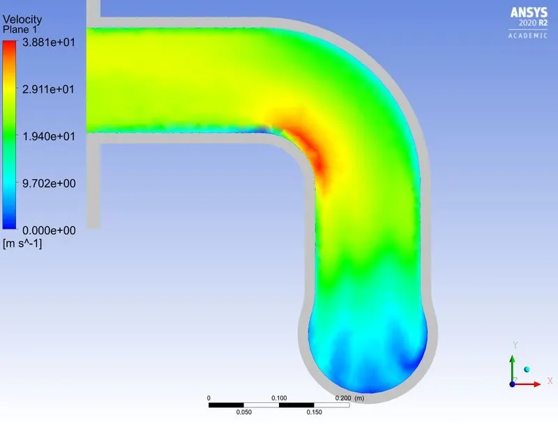
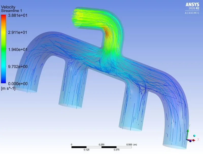
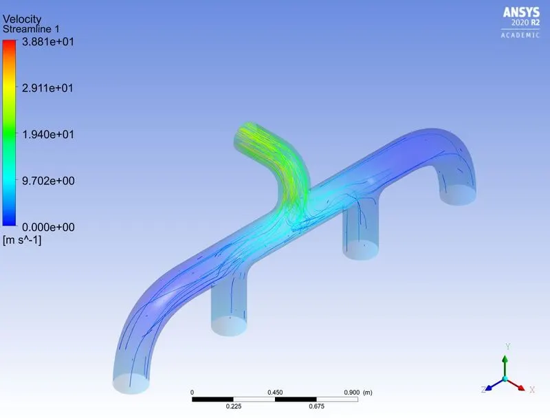
Velocity contour:
Temperature contour:
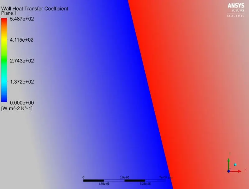
Area Average of Wall Heat Transfer Coefficient on inflation_layer
435.84 [W m^-2 K^-1]
Streamline:
To Verify the result:
Assuming the air as the fluid flowing in the pipe
For temperature t_air = 700k, from data book
Properties of air:
density = 0.524 `(kg)/m^3`
Kinematic viscosity = 63e-6`m^2/s`
Prandtl number = 0.678
Conductivity = 0.0521`W/m.K`
Reynold’s number = `(u.L)/v`
= `(5*0.166)/(63.03e-6)`
Thus, Re = `13.17e3`
For internal flow reynold’s number > 10000
Nusselt number Nu = `0.036〖Re〗^0.8 〖Pr〗^0.3`
Thus, Nu = 63.31378
We know that, Nu =`(h.D)/k`
Thus which gives h = 19.8591 `W/m^2.K`
thus the h = 20 `W/m^2.K` is used in the simulation
and it proves that the simulation is accurate.
(ii)as per the mass conservation law
we can say that the outlet velocity should be 4 times the inlet since there are 4 inlet and also the Inlet and outlet diameter are same.
Area Average of Velocity on outlet 25.2434 [`m s^-1`]
Thus the velocity is approximately 25 [`m s^-1`]
Conclusion:
Thus the simulation has successfully run in Ansys fluent.