Week 4 - CHT Analysis on Exhaust port

Objectives :

1. Give a brief description of why and where a CHT analysis is used.
2. Maintain the y+ value according to the turbulence model and justify the results. 
3. Calculate the wall/surface heat transfer coefficient on the internal solid surface & show the velocity & temperature contours in appropriate areas.
4. How would you verify if the HTC predictions from the simulations are right? On what factors does the accuracy of the prediction depend on?

 

Introduction and theory  :

Conjugate heat transfer is heat transfer between two different material like fluid and solid They exchange thermal energy  at interference between them. Electronic unit cooling and heating is widely used application of conjugate heat transfer.

The contemporary conjugate convective heat transfer model was developed after computers came into wide use in order to substitute the empirical relations of proportionality of heat flux to temperature difference with heat transfer coefficient which was the only tool in theoretical heat convection since the times of Newton. This model based on a strictly mathematically stated problem describes the heat transfer between a body and fluid flowing over or inside it as a result of the interaction of two objects. The physical processes and solutions of the governing equations are considered separately for each object in two subdomains. Matching conditions for these solutions at the interface provide the distributions of temperature and heat flux along with the body flow interface, eliminating the need for a heat transfer coefficient.

Why CHT analysis is used

CHT analysis accurately predict the actual behaviour of heat transfer by using the equations of heat transfer simultaneously.

CHT approach have advantage over finite element thermal analysis in that wall heat transfer coefficient and their local variation on surface are directly calculated on model rather than simplified calculations. CHT approach has benefits for these application where heat transfer is either non uniform or difficult to calculate

Where is CHT analysis is used ?

CHT is comes in widely used since computer are becomes normal these CHT analysis is first used in aerospace and nuclear reaction to thermal reacting products then it introduced in automotive industries then in food industries and after that it is common in pharma industries

Application of CHT:

1. internal combustion engine
2. Electronic components
3. compressors

Pre-Processing:

First of all we import the geometry in space claim and then we do the volume extract from prepare by selecting edges then we name those fluid and solid part as fluid volume and solid volume then we close our geometry as its part is over.

Opening the mesh we name the boundaries first and then create the base line mesh by using generate mesh after generating mesh we can see the inner and out part of geometry mesh doesn’t match each other so we go back one step by closing the mesh and opening geometry by reseting mesh. And turn the share topology as share from none.

By selecting the both volume we then create new component and then delete the empty component then we go to workbench and click on share which creates the single interface between solid and fluid  volume.

we create this above base line model so we can see first how the simulation is behaving and what are regions most affecting so later on during refinement we focus more on those areas so first we run all procedure on this base line mesh and then we run it on refined mesh

Going to mesh we again generate the mesh now after generating mesh if we can see the surface by zooming we can clearly see the conformal mesh meaning the fluid mesh and solid mesh is sharing there nodes with each other. This is the mesh we always need for the application of conjugate heat transfer. And as we reset the mesh before we have to name the boundaries again so we name it again and then generate the mesh

Setup :

1. K-omega:

As we dealing with convective heat transfer near the wall K omega works well where we want the result near the wall as compare to k epsilon because near wall it is not so good in precision and also we using y+ value between 0-5 as want result more accurate.

2. K-omega with sst:

Sst model is because it is good blended model like near wall its gives k omega advantage and away from wall it behaves like k-epsilon

3. Pressure Solver:

We chose pressure based solver because we are not considering any changes in density

4. Boundary condition :

In boundary condition we put inlet velocity as 25m/s with 700k as model is energy related and at outlet its pressure, wall convection we select convection

5. Maintaining y+ :

We maintain y+ value according to the model we are using so we put the desired y+ values as 4 (between 0-5) and as we dealing with the normal air so by putting its density and viscosity we get the estimated first layer thickness using the online y+ calculator. We get estimated first layer thickness as 5.4e-5m (0.054mm) which we used during inflation layer and according to our y+ range we select the model K-omega sst

Post-processing and results :

Solver: pressure based

Inlet velocity : 25m/s at 20wm2/k

At thermal condition of 700 k

Wall convection set to convection at 20wm2/k as heat transfer coeff and 300k as free stream temp

Fluid material is air along the solid made of aluminium

Viscous model : k-omega sst

 

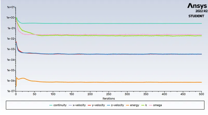
Fig 1.scaled residuals

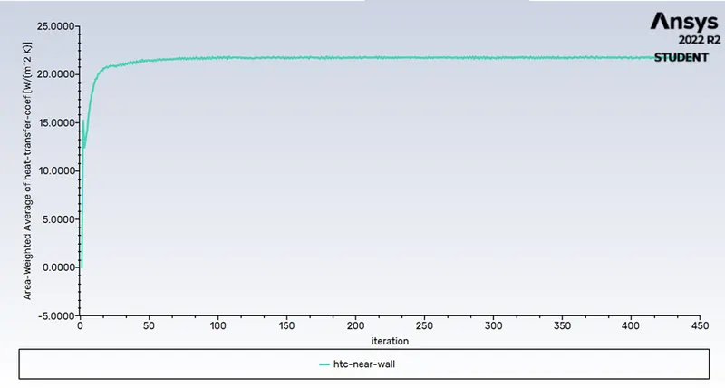
Fig 2. plot Heat transfer near wall shadow

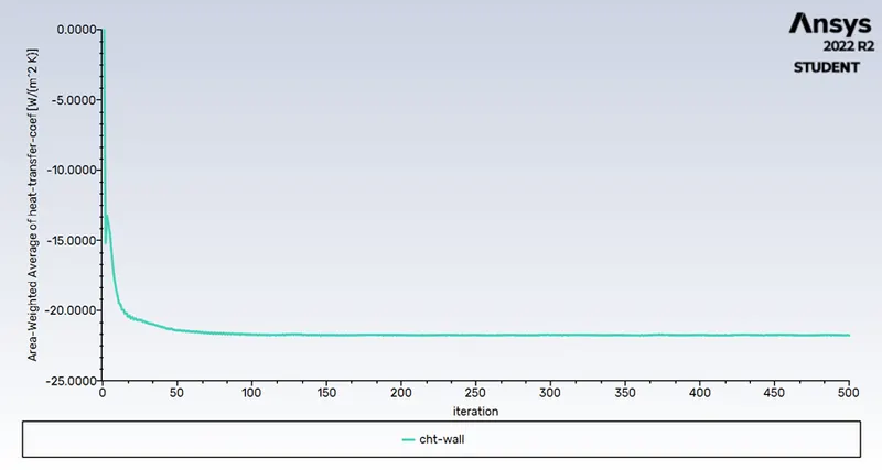
Fig 3. plot Heat transfer neat wall

 

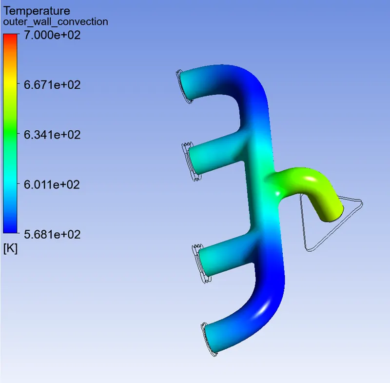
Fig4. Temperature contour along the pipe

 

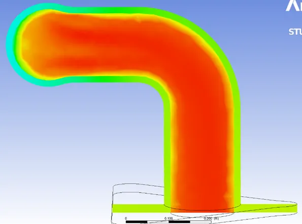
Fig 5. Temp contour at plane

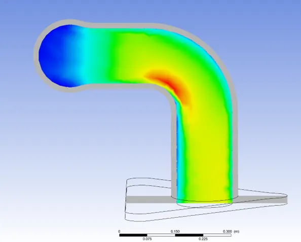
Fig 6. Velocity contour at plane

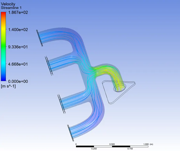
Fig 7. Velocity Streamline flow along pipe

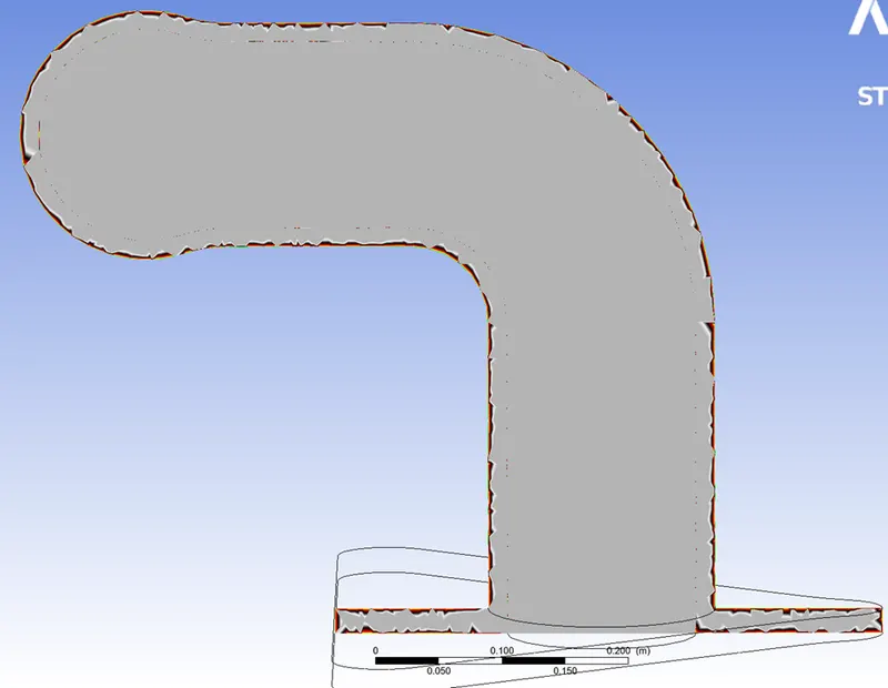
Fig 8. Heat transfer coefficient on the wall first layer

Results:

As per the simulation done on baseline model we there selected K epsilon model where we get that the k epsilon model didn’t behave more accurately near the wall and we want our important data near the wall so we select the k-omega SST model in actual simulation so that we get accurate and precise  simulation near the wall and  also due to SST model it behaves as k epsilon when condition is distant from wall. Also in main simulation we increase the mesh refinement where the part is most affected during simulation so we can get more accurate data at that particular point

Verification of HTC prediction from simulations :

According to Bernoulli’s mass conservation principle mass is conserved in our model which is clearly explained below

Let us assume the flow rate from each inlet as Q1,Q2,Q3,Q4 Respectively and Q5be the flowrate from exhaust manifold

Q1+Q2+Q3+Q4=Q5…….1

We have Q = rho*A*V

So equation will be,

A1V1+A2V2+A3V3+A4V4=A5V5

As it is an incompressible flow to compensate for mass flow velocity is increased and the overall mass flow rate is conserved

As velocity are high the Reynolds number at outlet manifold will be high

Nu = f(re,pr) for forced convection application

Nu= hD/k

From above formula Nu directly proportional to Re

Hence , Nu proportional to h

Therefore, Re is proportional to H

From our simulation it is  observed that at the bends the velocity is higher hence the Reynolds number will also be high there which has high heat transfer coefficient there fore prediction from our simulation are correct

 

Conclusion :

Factor that influence the prediction accuracy :

1. Mesh affect the accuracy of simulation more refined the mesh more the accuracy of simulation which we can also see in above contours and planes
2. We have to maintain the proper y+ value and the turbulence model both of them should be well synchronised with each other (we have to chose turbulence model based on y+ value range)
3. And in this simulation where the more focused is near wall so our Y+ value also be according to that which means 0-5 so we can chose the k-omega mode which is good near the wall problem