Week 4 - CHT Analysis on Exhaust port

CHT Analysis of an Exhaust port

Objectives:

• Maintain the y+ value according to the turbulence model and justify the results.
• Calculate the wall/surface heat transfer coefficient on the internal solid surface & show the velocity & temperature contours in appropriate areas.
• Enumerate the verification of HTC predictions and factors on which the accuracy of the prediction depends on.

CHT Analysis:

• Conjugate Heat Transfer Analysis is the simulation of any combination of heat transfer mechanisms such as conduction, convection, and radiation. In other words, Conjugate Heat Transfer (CHT) analysis type allows for the simulation of heat transfer between solid and fluid domains by exchanging thermal energy at the interfaces between them.
• Typical applications of CHT analysis are the simulation of heat exchangers, cooling of electronic equipment, and general-purpose cooling and heating systems.
• Heat transfer in solids and heat transfer in fluids are combined in the majority of applications. This is because fluids flow around solids, between solid walls, and solids are usually immersed in a fluid. An accurate description of heat transfer modes, material properties, flow regimes, and geometrical configurations enables the analysis of temperature fields and heat transfer. Such a description is also the starting point for a numerical simulation that can be used to predict conjugate heat transfer effects or to test different configurations in order, for example, to improve the thermal performances of a given application.

Exhaust Port-Geometry:

• Given geometry consists of 4 inlets and one outlet. (Ref. Fig a and b).

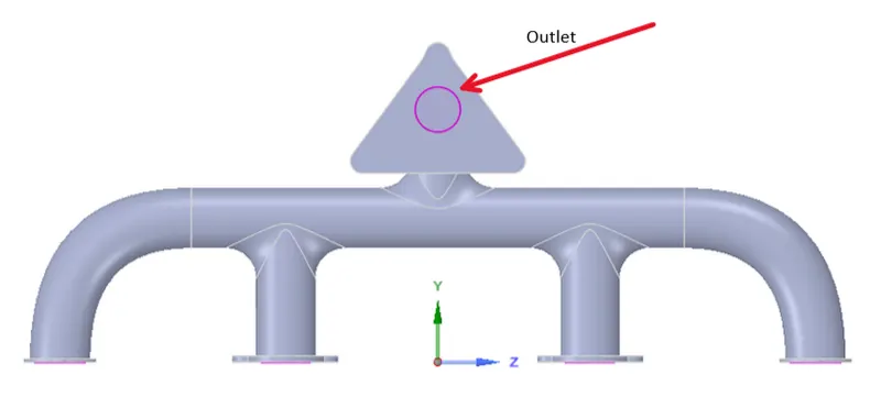
Fig a. Outlet

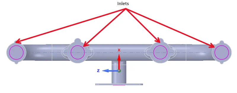
Fig b. Inlets

• Imported geometry is repaired from defects like split edges, duplicate edges, Gaps, Missing faces, etc. The region between fluid and solid is set to share topology such that the mesh is made conformal, which enables the transfer of computational information between regions.

Baseline Mesh: (Element size: 150mm, 137481 elements)

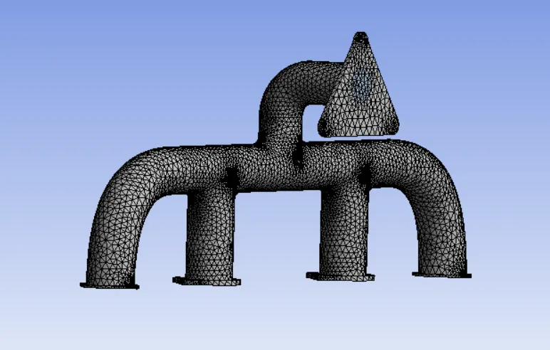
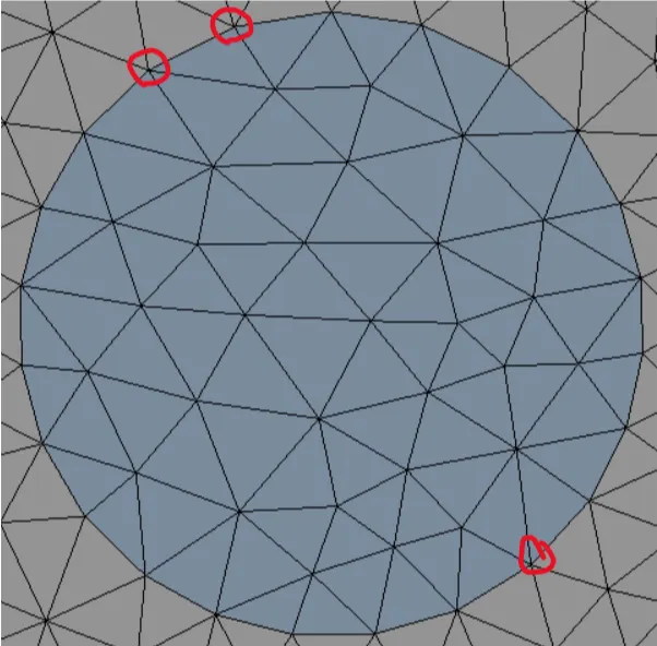
The vertices of fluid and solid volume are coincident at the interfaces and Hence a conformal mesh is created.

Simulation Setup:

Steady State - Pressure-based Solver

Energy Equation: ON

Viscous Model: K-epsilon

Materials

Fluid: Air, Solid: Aluminium

Boundary Conditions:

• Velocity Inlet: 5m/s, Temp: 700K
• Pressure Outlet
• Wall: Convection, HTC 20 W/m2K

Baseline results:

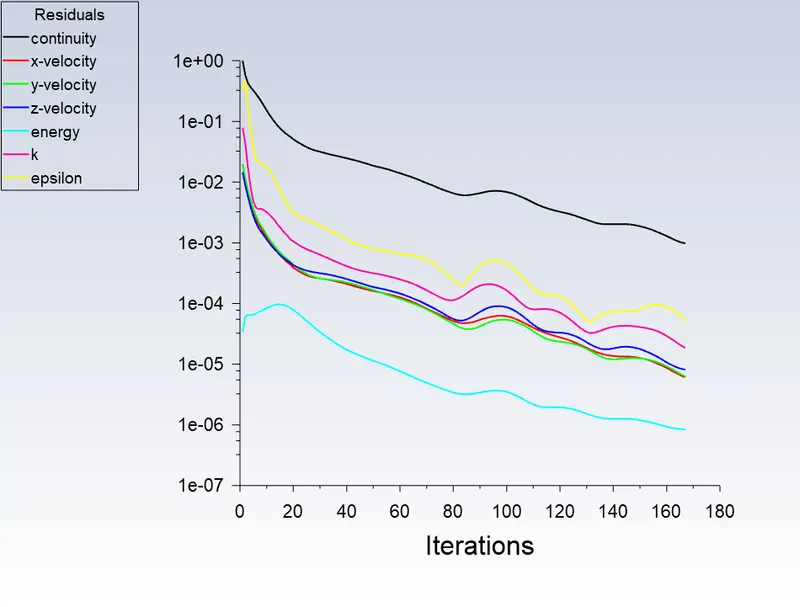
Residual:

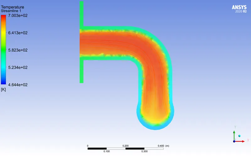
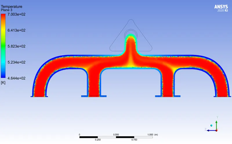
Temperature:

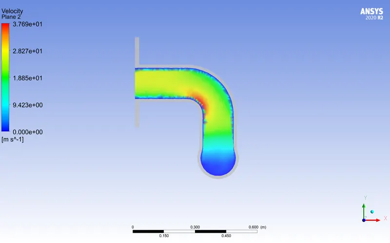
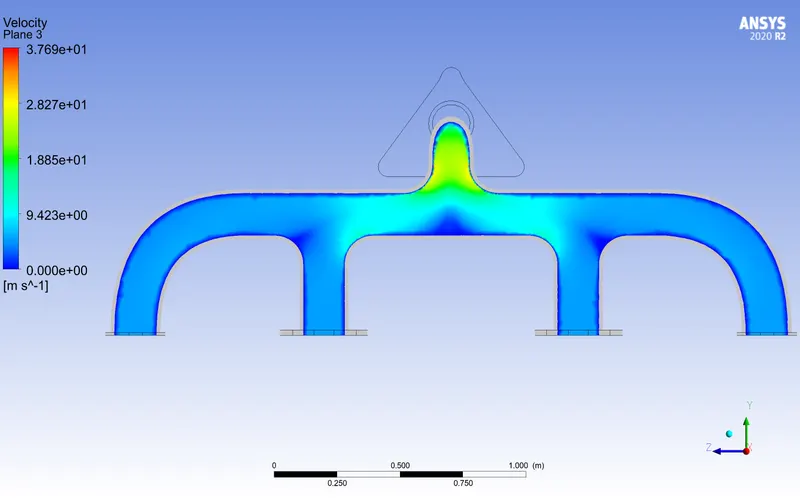
Velocity:

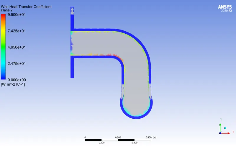
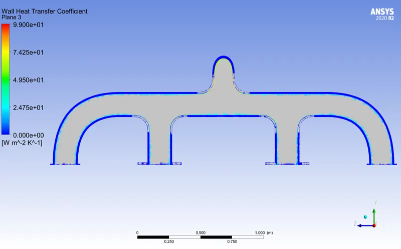
Heat Transfer Coefficient:

Refined Meshing:

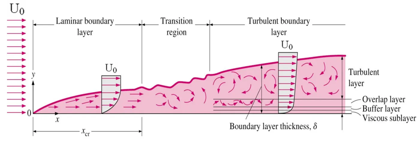
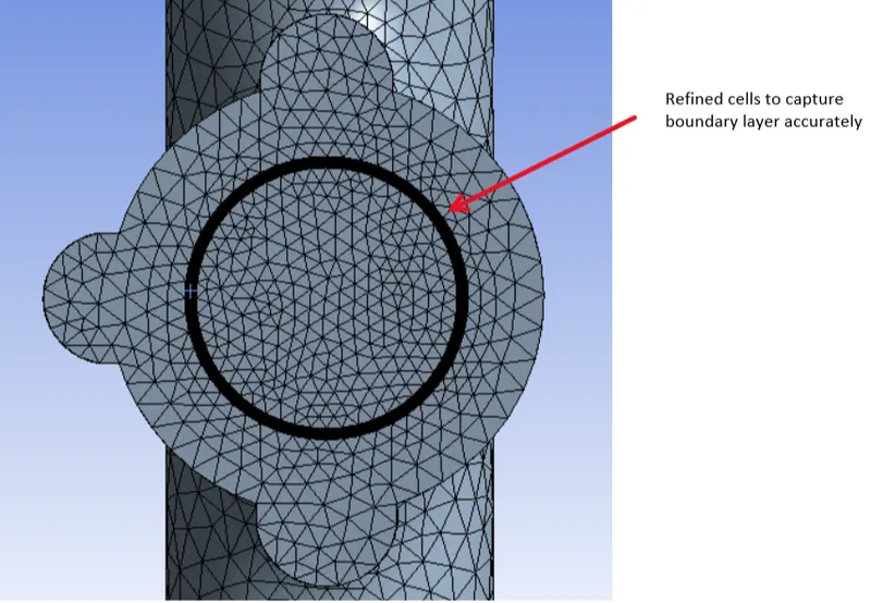
The value of is to distinguish different regions near the wall / viscous region. Let us try to understand this with an example. A fisherman uses a fishing net, a grid kind of structure, to trap the fish. If he is trying to catch medium to big-sized fishes, the grids in the net he uses are somewhat big, but if he is trying to trap even small-sized fishes then the grid size of the net should be small enough to capture them. In this case, even the large fish are also captured. Similarly, coming back to our case, if we intend to resolve the effects near the wall, i.e., in the viscous sub-layer, then the size of the mesh size should be small and dense enough near the wall so that almost all the effects are captured.

where is shear velocity, ρ - density (kg/m3), and μ is kinematic viscosity (kg/m-s) and target value is estimated based on the turbulence model used.

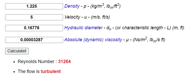
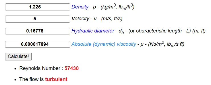
• First, lets calculate the Reynolds number,

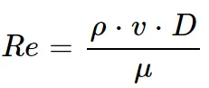
where,

Diameter (D) is considered to be 167.78mm, which is the average value of 4 inlet diameters

Viscosity mu =32.87e-06 (kg/m-s) (From Reference for 412deg C, near to 427deg C which is 700K)

Density rho=1.225 kg/m3

Velocity = 5 m/s

Re = (1.225*5*0.16778)/0.00003287 = 31264 (Turbulent Flow)

Verification:

• Skin Friction Coefficient for internal flows is,

Cf = 0.005941

• Wall shear stress,

tau = 0.5*0.005941*1.225*5*5 = 0.0909 kg /m-s^2

Here Uo is free stream velocity = 5 m/s

• Shear Velocity

Shear velocity, Ut = 0.2724 m/s

• Now finally, to calculate the first cell thickness, △y

y+ can be > 30, (Since k-ε is the turbulence model due to high Reynolds number)

First cell thickness, △y= 0.002955 m (Here y+ = 30)

Refined mesh is created as follows; (Element size:10mm, 961844 elements)

Simulation Setup:

Same as the Baseline case but with K-epsilon Enhanced Wall Treatment to capture wall accurately.

Results:

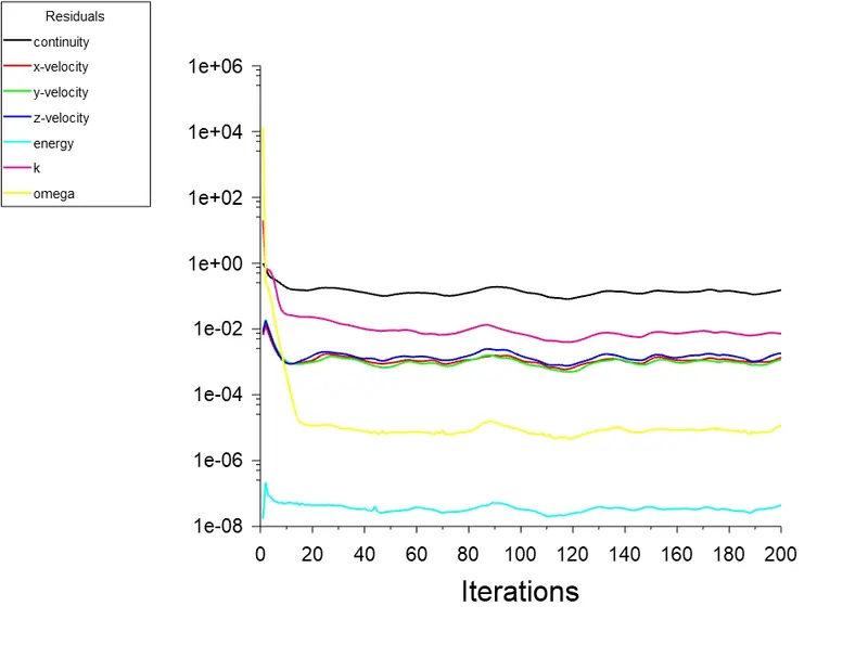
Residuals:

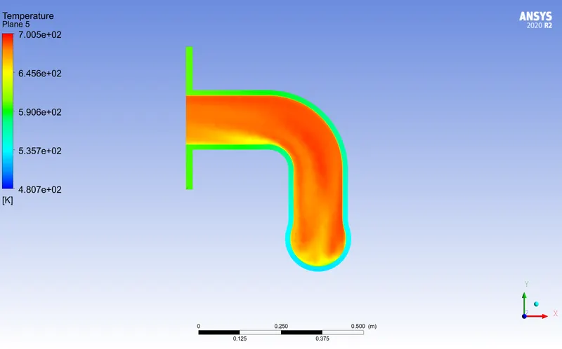
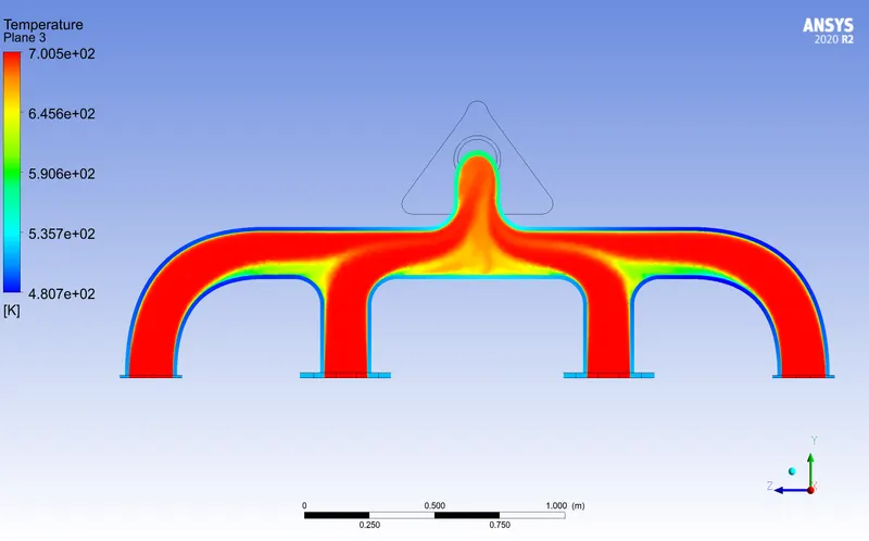
Temperature:

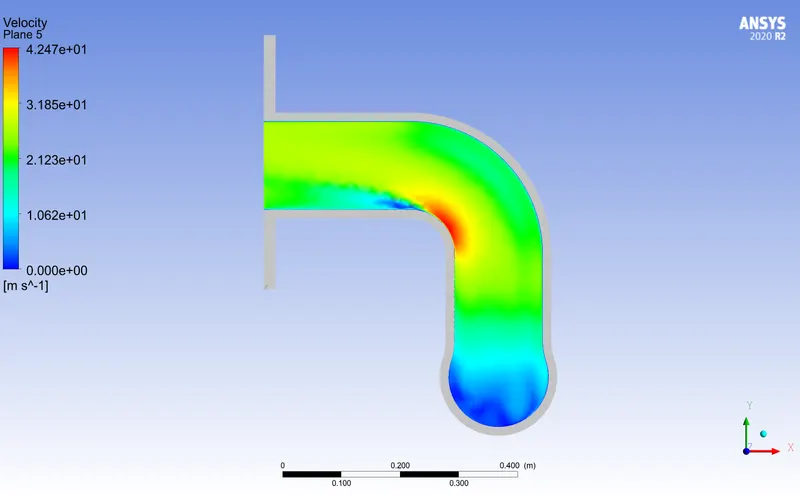
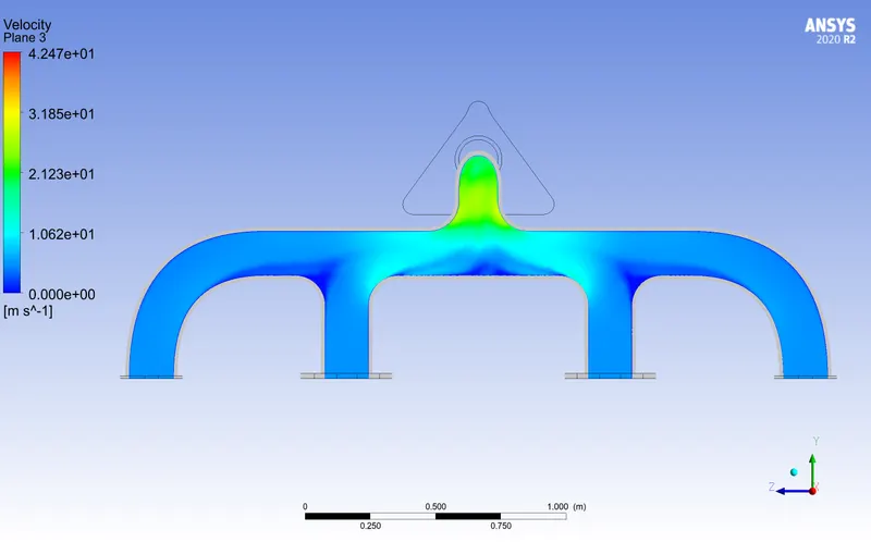
Velocity:

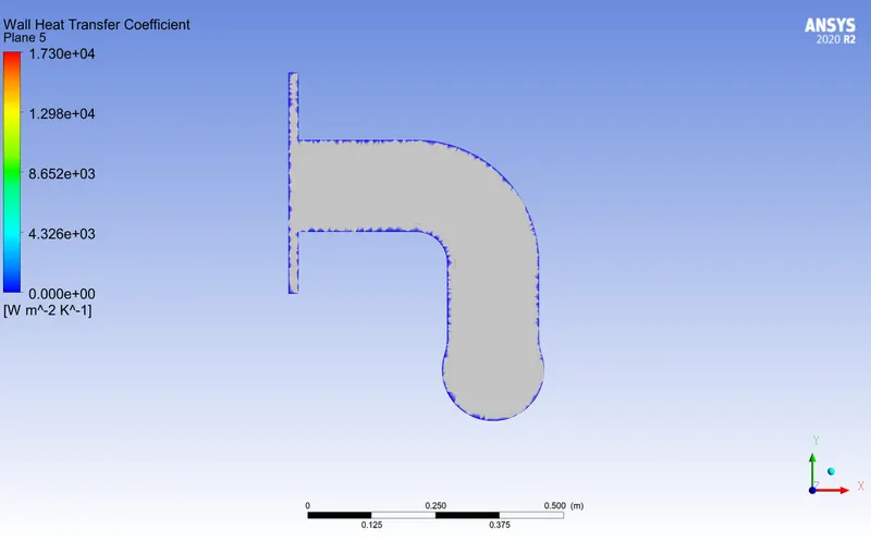
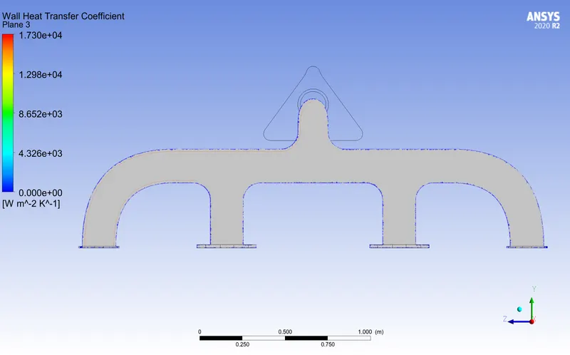
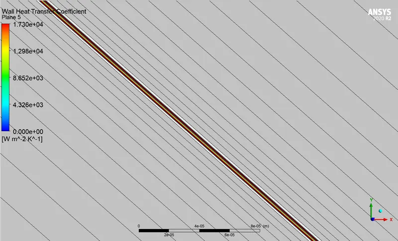
HTC:

Inferences:

Parameters	Baseline	Refined
Velocity m/s	37.6	42.4
Max. Temperature K	700.3	700.5
Min. Temperature K	464.4	480.7
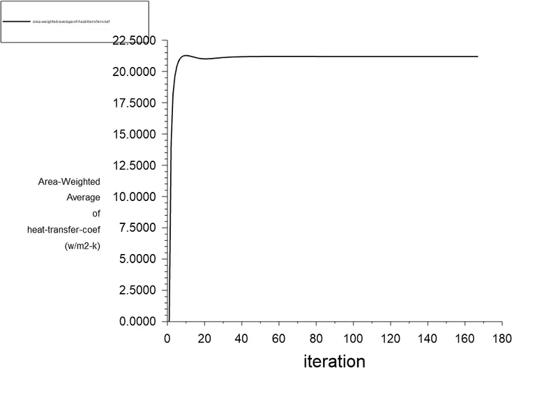
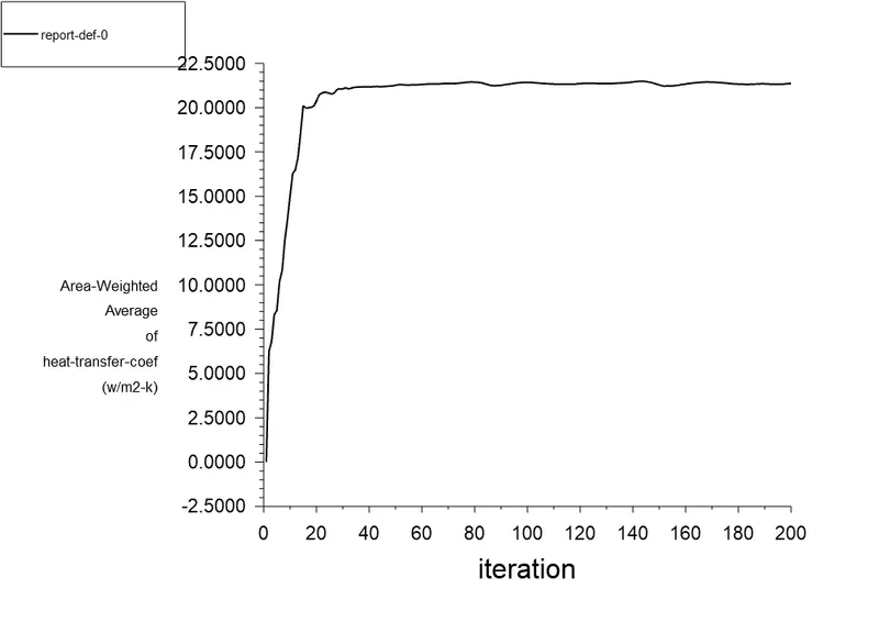
HTC W/m2K	21.19	21.36

• Between the Refined and Baseline mesh setup, maximum temperature variation is insignificant. However, the temperature at the walls, which corresponds to minimum temperature has a major deviation with 464.4K in the baseline case and 480.7K in the refined case. This is due to the fact that the mesh is refined at the fluid-solid interface. Hence, a major difference in the minimum temperature.
• Velocity is maximum near the outlet where all the fluid merges to exit. The peak velocity is near the walls and not in the center of the flow. Due to wall treatment in refined case, there is a considerable deviation in maximum velocity from baseline setup.

Verification of HTC predictions from simulations:

(i) Prandl Number:

The Prandtl number (Pr) is a dimensionless number defined as the ratio of momentum diffusivity to thermal diffusivity.

= 0.795

: specific heat, 1075 ( J/(kg·K)) [ref.3]

: dynamic viscosity, 1.7894e-05 ( N s/m²) [As per FLUENT material data]

: thermal conductivity of Air, 0.0242 (W/(m·K))

(ii) Dittus–Boelter equation:

The Dittus–Boelter equation (for turbulent flow) as introduced by W.H. McAdams, is an explicit function for calculating the Nusselt number. It is easy to solve but is less accurate when there is a large temperature difference across the fluid. It is tailored to smooth tubes, so use for rough tubes (most commercial applications) is cautioned.

= 137.76

for the fluid being heated, and for the fluid being cooled

Here Re,

(iii) Nusselt Number:

Nusselt Number is the ratio of convective to conductive heat transfer across a boundary.

In terms of diameter,

, = 19.87 (Analytical)

Here D = 0.16778 m

Area Weighted Average of HTC = 21.19 (Numerical-Baseline)

Area Weighted Average of HTC = 21.36 (Numerical-Refined)

Error = |Actual - Estimated|/Actual *100 = 7.49%

Factors affecting HTC:

There are multiple factors that affect HTC. They are;

• Analytically, the correct estimation of the Reynolds number, Prandl, and Nusselt number is essential.
• The method or relation used to derive the HTC has to be valid for the physics being solved.
• For the correct estimation of the above parameters, a geometry that is accurate to the actual scenario has to be used.
• Properties of Materials also play a crucial role as Thermal conductivity influences the estimation of HTC.
• If all the above items are accurate, the setup of the simulation, such as the choice of Turbulence model and refinement of Mesh along the walls using proper Y+, is essential.

References:

[1] https://www.engineeringtoolbox.com/air-absolute-kinematic-viscosity-d_601.html

[2] https://www.learncax.com/knowledge-base/blog/by-category/cfd/basics-of-y-plus-boundary-layer-and-wall-function-in-turbulent-flows

[3] https://www.engineeringtoolbox.com/air-specific-heat-capacity-d_705.html

[4] https://en.wikipedia.org/wiki/Nusselt_number