Week 4 - CHT Analysis on Exhaust port

AIM:

• The aim of this assignment is to perform a Conjugate Heat Transfer analysis and simulate flow inside an Exhaust port.

OBJECTIVE:

The objectives of this assignment are:

• To give a brief description about Conjugate Heat Transfer (CHT) analysis and where and why it is used.
• To perform CHT analysis on Exhaust Port.
• To select a proper turbulence model and maintain the correct Y plus value.
• To compute the Velocity, Temperature, Heat transfer coefficient contours and Y plus plots and other required contours and plots to show the results of the CHT analysis on the Exhaust Port.
• To validate the result and verify if the HTC predictions from the simulations are right or not.
• To state on what factors does the accuracy of the prediction depend on.

INTRODUCTION:

CONJUGATE HEAT TRANSFER ANALYSIS:

• The Conjugate Heat Transfer (CHT) analysis type allows for the simulation of heat transfer between solid and fluid domains by exchanging thermal energy at the interfaces between them. Typical applications of this analysis type exist as, but are not limited to, the simulation of heat exchangers, cooling of electronic equipment, and general-purpose cooling and heating systems. Efficiently combining heat transfer in fluids and solids is the key to designing effective coolers, heaters, or heat exchangers.
• The fluid usually plays the role of energy carrier on large distances. Forced convection is the most common way to achieve high heat transfer rate. In some applications, the performances are further improved by combining convection with phase change (for example liquid water to vapour phase change). Even so, solids are also needed, in particular to separate fluids in a heat exchanger so that fluids exchange energy without being mixed.
• The temperature field and the heat flux are continuous at the fluid/solid interface. However, the temperature field can rapidly vary in a fluid in motion: close to the solid, the fluid temperature is close to the solid temperature, and far from the interface, the fluid temperature is close to the inlet or ambient fluid temperature. The distance where the fluid temperature varies from the solid temperature to the fluid bulk temperature is called the thermal boundary layer. The thermal boundary layer size and the momentum boundary layer relative size is reflected by the Prandtl number. For the Prandtl number to equal 1, thermal and momentum boundary layer thicknesses need to be the same. A thicker momentum layer would result in a Prandtl number larger than 1. Conversely, a Prandtl number smaller than 1 would indicate that the momentum boundary layer is thinner than the thermal boundary layer. The Prandtl number for air at atmospheric pressure and at 20°C is 0.7. That is because for air, the momentum and thermal boundary layer have similar size, while the momentum boundary layer is slightly thinner than the thermal boundary layer. For water at 20°C, the Prandtl number is about 7. So, in water, the temperature changes close to a wall are sharper than the velocity change.

Heat transfer in solids and heat transfer in fluids are combined in the majority of applications. This is because fluids flow around solids or between solid walls, and because solids are usually immersed in a fluid. An accurate description of heat transfer modes, material properties, flow regimes, and geometrical configurations enables the analysis of temperature fields and heat transfer. Such a description is also the starting point for a numerical simulation that can be used to predict conjugate heat transfer effects or to test different configurations in order, for example, to improve thermal performances of a given application.

Application:-

The conjugate heat transfer methods have become a more powerful tool for modeling and investigating nature phenomena and engineering systems in different areas ranging from aerospace and nuclear reactors to thermal goods treatment and food processing from the complex procedures in medicines to ocean thermal interaction in metrology.

CHT in recent years has significantly improved the cooling performance of electronic equipment such as the design of heat sinks and the design of heat exchangers for the waste treatment plant. One such application of CHT is the exhaust port system.

Solving and modeling approach:-

1.The exhaust port was modeled into the Spaceclaim.

2.The exhaust port is a three-dimensional model containing four inlets and one outlet. Despite having isothermal boundary conditions and a uniform flow rate at the four inlets, the model cannot be cut into two halves to save computational time because of its asymmetrical nature. Therefore the whole model is discretized and is considered for meshing.

3.CHT analysis requires both the solid and the liquid volume under consideration, Spaceclaim gives an option of volume extract for selecting edges for fluid volume.

4.Both the solid volume and liquid volume are copied into one component.

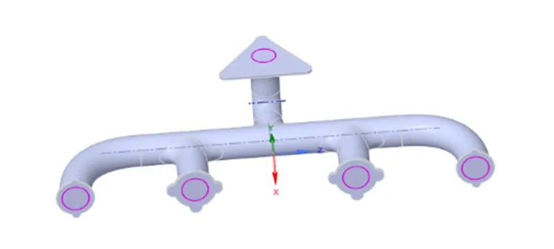
5.Share topology is created.

6.Spaceclaim gives an option for share coincident topology, when share coincident topology is selected and executed, the mesh from the fluid volume and the solid volume are said to be conformal with each other which is a requirement for CHT analysis.

7.The exhaust port is loaded into the meshing window and then simulated for baseline mesh and the refined mesh.

8.The named selections are created ( inlet, outlet, outer wall convection)

9.The necessary contour images and graphs are studied to understand the behavior of temperature, velocity, and surface heat transfer coefficient at the interface.

Pre-processing and solver setting :-

Baseline mesh :-

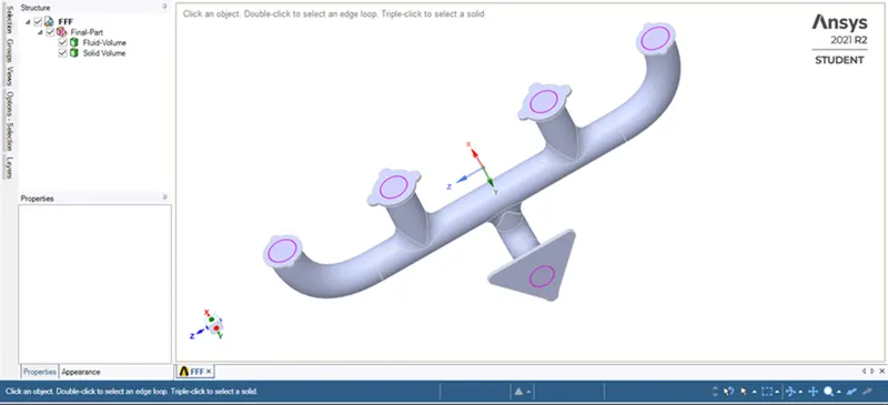
The geometry is loaded into Spaceclaim.

Fluid volume extraction :-

It is the process of extracting the fluid volume from the solid volume.

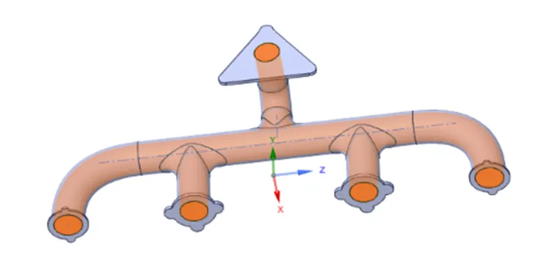
Share topology:-

Meshing:-

It is the process of discretizing the geometry into a small number of volumes containing nodes. Since the geometry is complex and the mesh is unstructured therefore the finite volume scheme is used as a discretization scheme.

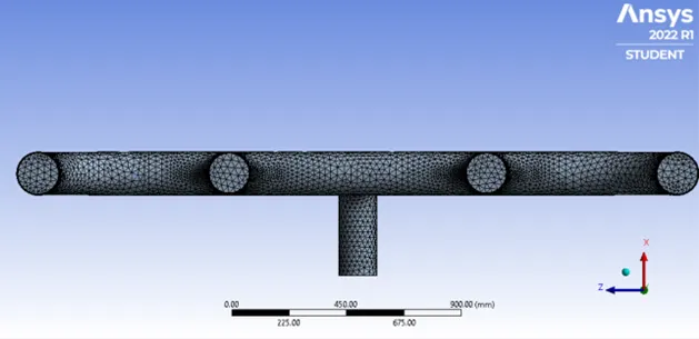
Mesh statistics:-

Number of elements	135525
Number of nodes	27218

Setting up of physics and boundary conditions:-

The geometry orientation in the setup window. The blue-colored lines are inlet, and the red-colored lines are outlet.

Set up:-

The different boundary conditions are listed below

• Inlet boundary condition

1. Type: Velocity inlet
2. Velocity magnitude :5m/sec
3. Temperature: 700K

• Outlet boundary condition

1. Type: Pressure outlet
2. Gauge pressure: 0Pa

• Outer wall convection

1. Type: wall
2. Thermal condition: convection
3. Heat transfer coefficient: 20W/m^2*K
4. The rest boundary condition values are set up as default values in ANSYS-FLUENT.

• Energy equation: It is turned on.
• Viscous model: It is set to k−ωSST

Material properties

Fluid

• Material Name: Air
• Density: 1.225kg/m^3
• Specific heat: 1006.43J/kg*K
• Thermal conductivity: 0.0242W/m*K
• Viscosity: 1.7894e−05kg/m−sec

Solid

• Material Name: Aluminium
• Specific heat: 871J/kg*K
• Thermal conductivity: 202.4W/mK.

SIMPLE METHOD:-

Residual plot:-

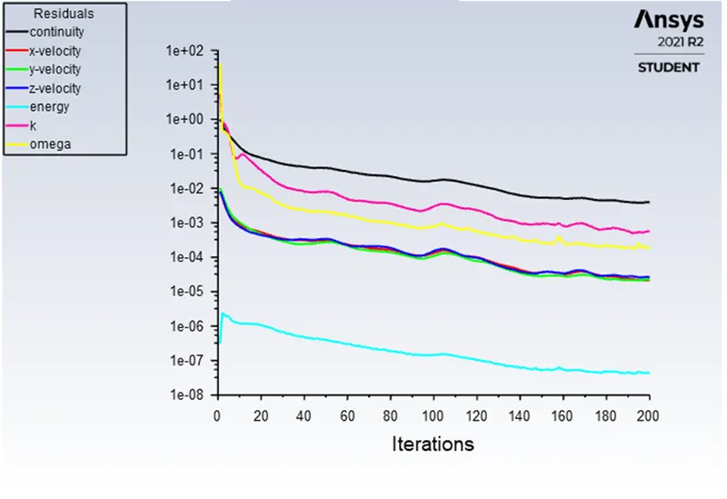
Surface heat transfer coefficient:-

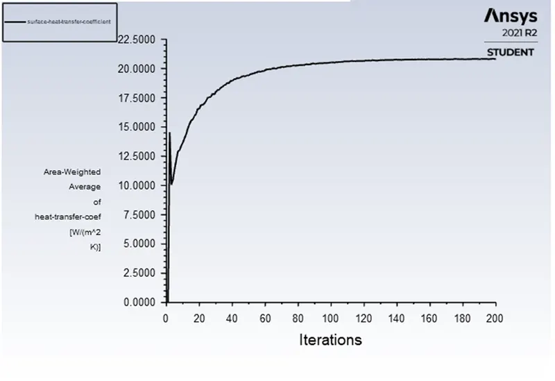
Surface heat transfer coefficient value:- 21.906122 W/m^2*K

After same we can another value of Surface heat transfer coefficient :- 22.W/m^2*K

CHT analysis of exhaust port with finermesh :-

First refinement :-

Element size: 90mm

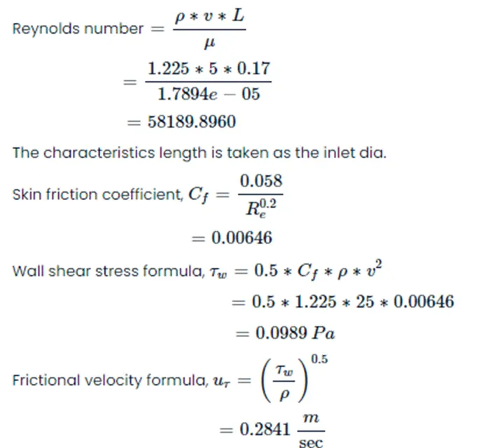
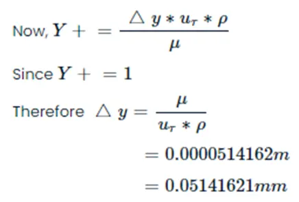
Since the value of the heat transfer coefficient takes the value of the first cell near the wall, so it can be inferred that the Y+ value will be in the viscous sub-layer which is taken to be 1.

Steps involved in calculating the first cell height.

Inflation:-

Number of inflation layer: 6

Growth rate: 1.2

Inflation option: First layer thickness

First layer thickness: =0.05141621mm

Captured curvature is set to yes

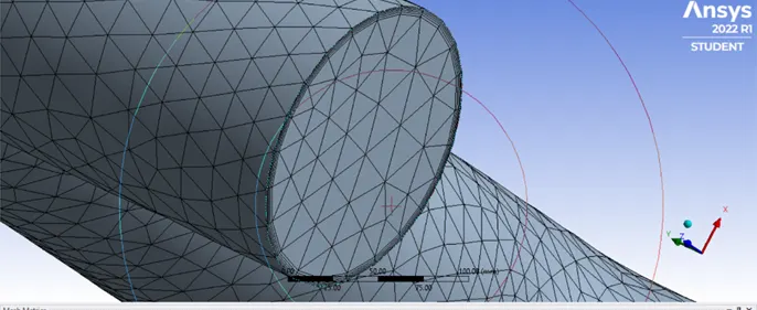
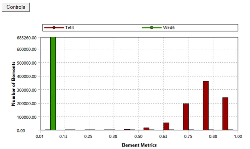
Mesh Quality:-

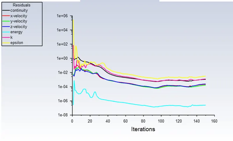
Residual plot:-

Surface heat transfer coefficient:-

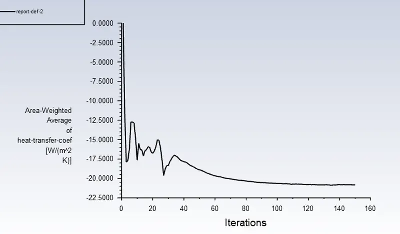
Mesh statistics and surface heat transfer coefficient:-

Element size	90 mm
Number of elements	280922
Number of nodes	100407
Y+	1
First cell height	0.0514 mm
Heat transfer coefficient	21.4865W/m^2*K

Results:-

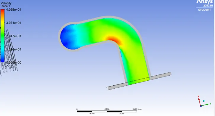
The temperature along plane-1 located at the exhaust section of the port:-

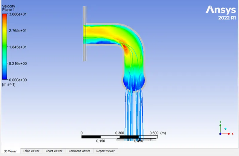
The velocity along plane-1 located at the exhaust section of the port:-

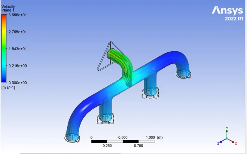
Streamline representation of velocity:-

CONCLUSION:

• From the above experiment we can conclude that the correct of Y+ value will give the accurate heat transfer coefficient.
• From the temperature contour we can notice that the temperature at the outlet side is more than the inlet side.
• This happens because of conservation of mass i.e. the mass flow rate of fluid exiting out of the port should be equal to the sum of all mass flow rate of the fluid coming in from the inlet side.
• Conservation of mass = mo=mi1+mi2+mi3+mi4mo=mi1+mi2+mi3+mi4
• Due to the conservation of mass the velocity near the outlet side will be more than the inlet side and this can be clearly seen from the velocity plots.
• Due to high velocity at that position the Reynold's number will also be high which in turn increases the Nusselt number and thus the value of heat transfer coefficient near the outlet region increases.
• This increase in the value of the surface heat transfer coefficient at the outlet region can be observed from the contour provided above.
• To validate the results of the heat transfer coefficient obtained we have performed the simulation by refining the mess and can be observed that the value of the heat transfer coefficient remains almost same.
• From the above Wall Y plus plots it can be clearly observed that the value of Y Plus is maintained between the 0 to 5 region which is the correct range for the K-Omega turbulence model.
• To get the accurate value of heat transfer coefficient we must select the proper turbulence model and the correct Y plus value to get the correct first layer thickness value.