Conjugate Heat Transfer analysis in exhaust port.

1. Give a brief description of why and where a CHT analysis is used.
2. Maintain the y+ value according to the turbulence model and justify the results.
3. Calculate the wall/surface heat transfer coefficient on the internal solid surface & show the velocity & temperature contours in appropriate areas.
4. How would you verify if the HTC predictions from the simulations are right? On what factors does the accuracy of the prediction depend?

Solution:

What is CHT?

CHT is an acronym for Conjugate Heat Transfer and the Conjugate Heat Transfer (CHT) analysis type allows for the simulation of heat transfer between solid and fluid domains by exchanging thermal energy at the interfaces between them. Typical applications of this analysis type exist as, but are not limited to, the simulation of heat exchangers, cooling of electronic equipment, and general-purpose cooling and heating systems.

Where it is used?

Why it is used?

Conjugate heat transfer corresponds with the combination of heat transfer in solids and heat transfer in fluids. In solids, conduction often dominates whereas, in fluids, convection usually dominates. Conjugate heat transfer is observed in many situations. For example, heat sinks are optimized to combine heat transfer by conduction in the heat sink with the convection in the surrounding fluid. There are different ways that heat transfer can take place in a different medium.

Heat Transfer by Solids and Fluids

Heat Transfer in a Solid

In most cases, heat transfer in solids, if only due to conduction, is described by Fourier’s law defining the conductive heat flux, q, proportional to the temperature gradient: .

For a time-dependent problem, the temperature field in an immobile solid verifies the following form of the heat equation:

Heat Transfer in a Fluid

Due to the fluid motion, three contributions to the heat equation are included:

1. The transport of fluid implies energy transport too, which appears in the heat equation as the convective contribution. Depending on the thermal properties on the fluid and on the flow regime, either the convective or the conductive heat transfer can dominate.
2. The viscous effects of the fluid flow produce fluid heating. This term is often neglected, nevertheless, its contribution is noticeable for fast flow in viscous fluids.
3. As soon as a fluid density is temperature-dependent, a pressure work term contributes to the heat equation. This accounts for the well-known effect that, for example, compressing air produces heat.

Accounting for these contributions, in addition to conduction, results in the following transient heat equation for the temperature field in a fluid:

Conjugate Heat Transfer Applications

Effective Heat Transfer

Efficiently combining heat transfer in fluids and solids is the key to designing effective coolers, heaters, or heat exchangers.

The fluid usually plays the role of energy carrier on large distances. Forced convection is the most common way to achieve a high heat transfer rate. In some applications, the performances are further improved by combining convection with phase change (for example liquid water to vapor phase change).

Even so, solids are also needed, in particular, to separate fluids in a heat exchanger so that fluids exchange energy without being mixed.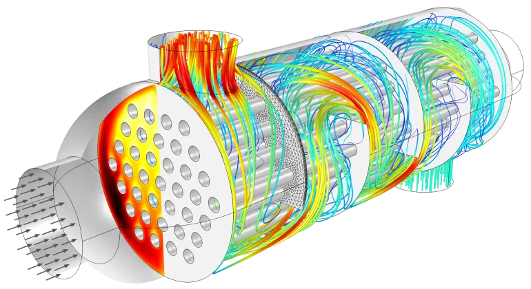

Flow and temperature field in a shell and tube heat exchanger illustrating heat transfer between two fluids separated by the thin metallic wall.

Heat sinks are usually made of metal with high thermal conductivity (e.g. copper or aluminum). They dissipate heat by increasing the exchange area between the solid part and the surrounding fluid.

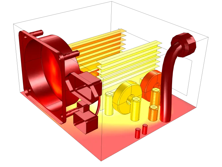
Temperature field in a power supply unit cooling due to an airflow generated by an extracting fan and perforated grille. Two aluminum fins are used to increase the exchange area between the flow and the electronic components.

Energy Savings

Heat transfer in fluids and solids can also be combined to minimize heat losses in various devices. Because most gases (especially at low pressure) have small thermal conductivities, they can be used as thermal insulators… provided they are not in motion. In many situations, gas is preferred to other materials due to its low weight. In any case, it is important to limit the heat transfer by convection, in particular by reducing the natural convection effects. Judicious positioning of walls and use of small cavities helps to control the natural convection. Applied at the micro-scale, the principle leads to the insulation foam concept where tiny cavities of air (bubbles) are trapped in the foam material (e.g. polyurethane), which combines high insulation performances with lightweight.

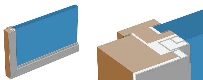
Window cross-section (left) and zoom-in on the window frame (right).

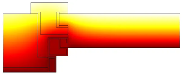
The temperature profile in a window frame and glazing cross-section from ISO 10077-2:2012

Fluid and Solid Interactions

Fluid/Solid Interface

The temperature field and the heat flux are continuous at the fluid/solid interface. However, the temperature field can rapidly vary in a fluid in motion: close to the solid, the fluid temperature is close to the solid temperature, and far from the interface, the fluid temperature is close to the inlet or ambient fluid temperature. The distance where the fluid temperature varies from the solid temperature to the fluid bulk temperature is called the thermal boundary layer. The thermal boundary layer size and the momentum boundary layer relative size are reflected by the Prandtl number : for the Prandtl number to equal 1, thermal and momentum boundary layer thicknesses need to be the same. A thicker momentum layer would result in a Prandtl number larger than 1. Conversely, a Prandtl number smaller than 1 would indicate that the momentum boundary layer is thinner than the thermal boundary layer. The Prandtl number for air at atmospheric pressure and at 20°C is 0.7. That is because, for air, the momentum and thermal boundary layer have similar sizes, while the momentum boundary layer is slightly thinner than the thermal boundary layer. For water at 20°C, the Prandtl number is about 7. So, in water, the temperature changes close to a wall are sharper than the velocity change.

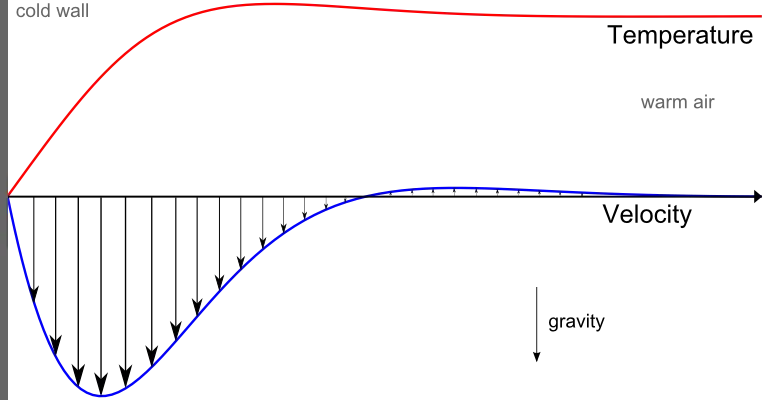
Normalized temperature (red) and velocity (blue) profile for natural convection of air close to a cold solid wall.

Now we are going to perform a few simulations on the basis of the above explanation on CHT. Here we are going to take a . STEP file of an Exhaust port where we are going to simulate conjugate heat transfer.

we are going to run a space claim and export our geometry in there and begin building for mesh.

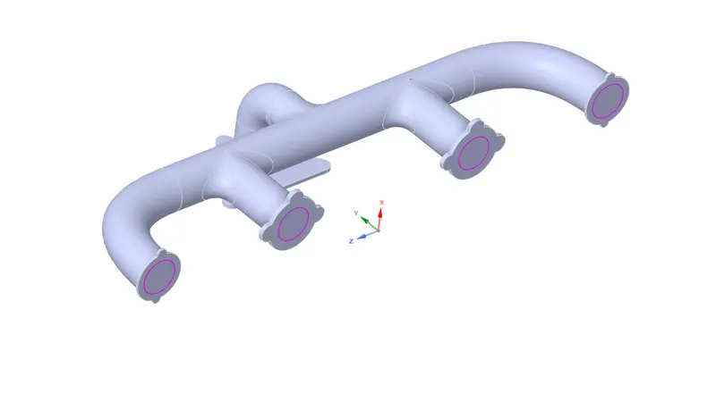
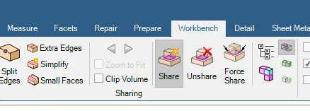
Now we observed that the solids need to share the information as a single unit so we are made this geometry in sharing topology scheme which consists of 2 different domains the solid and fluid volume. a tool we used in the space claim is SHARE.

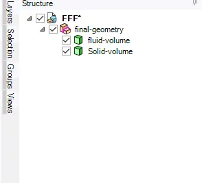
Now that we have developed the geometry, we are going to mesh the whole geometry for simulations.

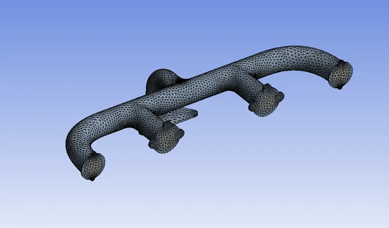
as we can see the mesh has been generated but we have refined it yet before running. We gonna do it few upcoming steps but let's see how the domain is when the shared topology is been active and the 2 bodies going to share information with each other.

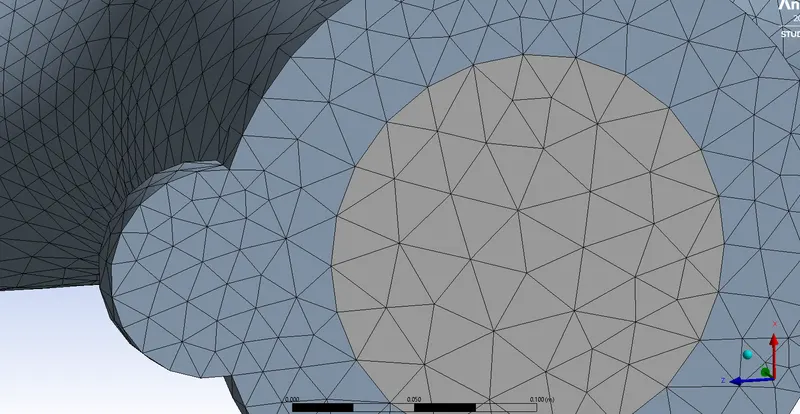
Now before we jump into the fluent to run some simulation we are going to refine the above mesh. and to validate the result we have checked Y+ of different turbulence modeling.

so now that we have taken into consideration that we will have different Y+ values of different turbulent modeling we are going to determine the refining strategy. However, we engineers always get complicated when it comes to calculating different numerical values which is time-consuming, therefore we have to reduce time effort we have an online calculator of determining the Initial boundary layer with targeted Y+. So different turbulence modeling have different y+ and according to that, we are going to perform refinement in INFLATION LAYER.

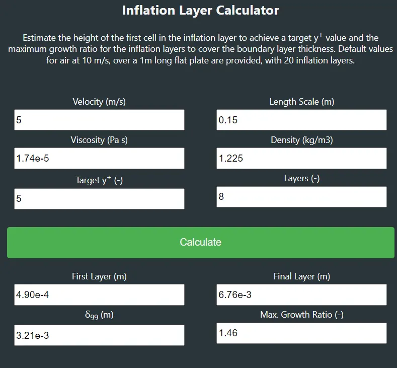
The Online calculator represents as :

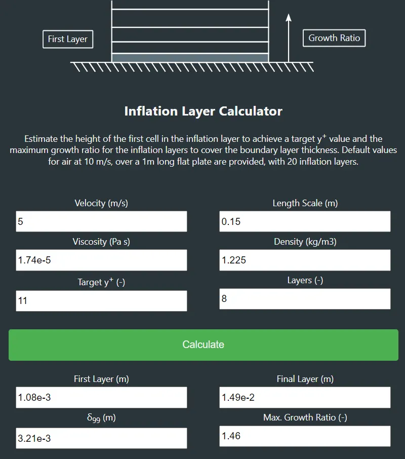
so for 1st Y+ is 11 we have taken and then going to produce the mesh accordingly with the first layer as 1.08e-3 m.

And we can calculate the Y+ values in CFD-Post where we plot the features turbulence/ wall Y+ with a vector.

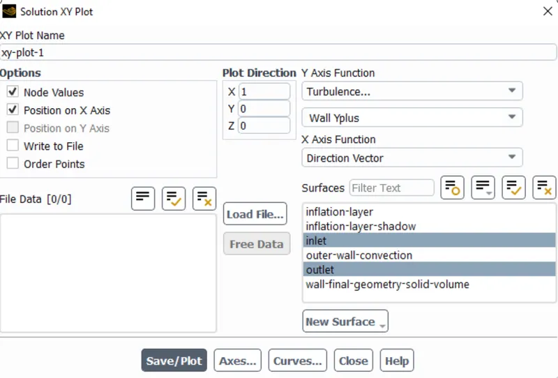
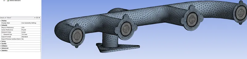
this is the mesh we created and the wall Yplus we got plotted as:

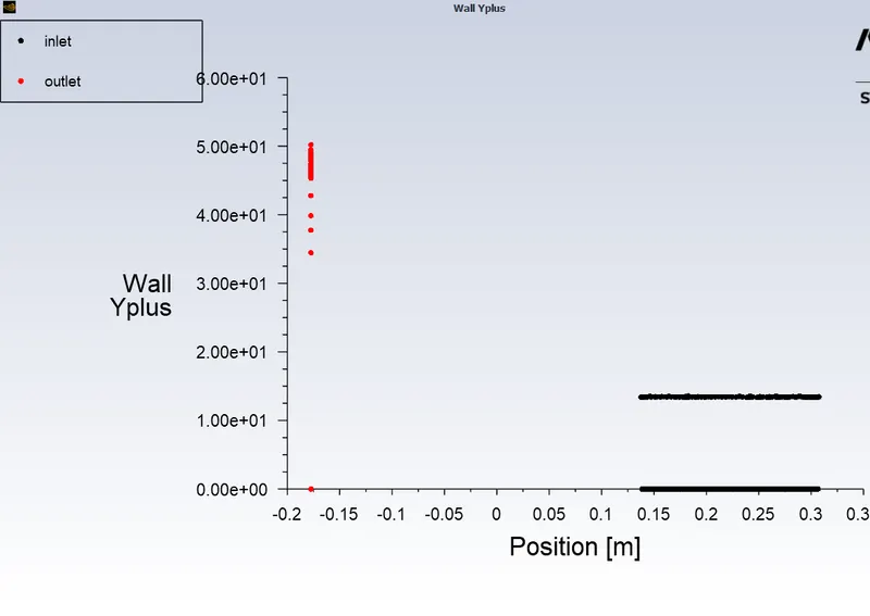
It seems the Y+ is below 11, the values we took to determine the first layer thickness and the value is around 5e+1. Y+ = 5 < 11. So here we concur that we used standard wall function for near-wall treatment. Which is exactly what we did. The value didn't give us the exact results here but it was around 11. so it's just around the given value.

so Y+ value for validation is 5 whereas the given value was 11. And we used K-epsilon realizable model.

Now for our 2nd Y+ we have taken as 50 and then going to produce the mesh accordingly with the first layer as 4.90e-3 m.

with elements cell count of 302222

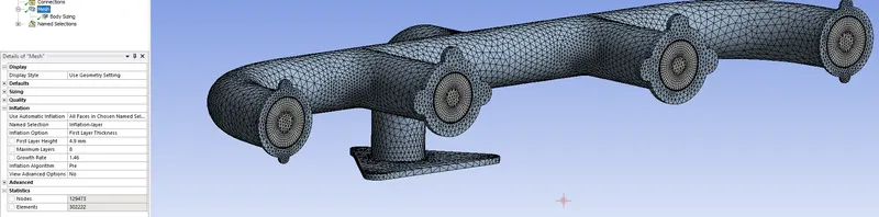
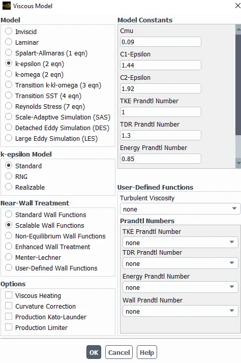
This time we are going to use scalable wall function for near-wall treatment. The value didn't give us the exact results here but it is more than 50. 30<Y+< 300. so here Y+ is 2.00e+02 i.e 200

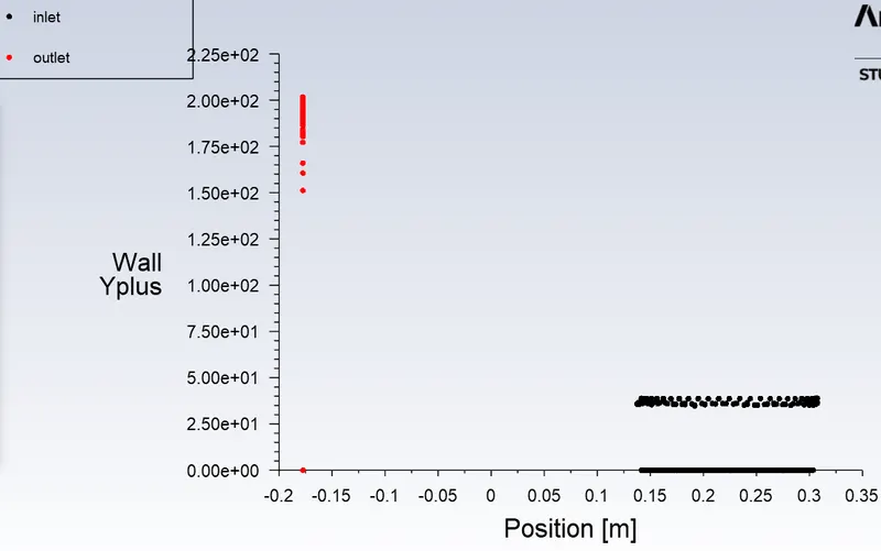
Use K-Epsilon model with scalable wall functions (default option in new version of Fluent). It will keep the Y+ above 11.06 so that it does not suffer the limitation of old standard wall functions. Moreover now you can carry the successive refinement of mesh, which was not possible with standard WFs.

Here for our 3rd Y+ value we have 5 and then going to produce the mesh accordingly with the first layer as 4.90e-4 m.

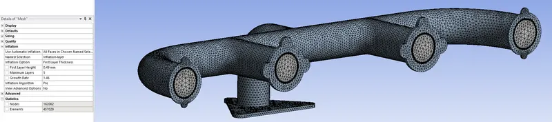
with only 457209 cells count we are just very close to the limited cell counts for our academic license of FLUENT and preumbaly our last case for selecting the turbulence modeling for any Y+.

and now had Y+ as 5 in the calculator.

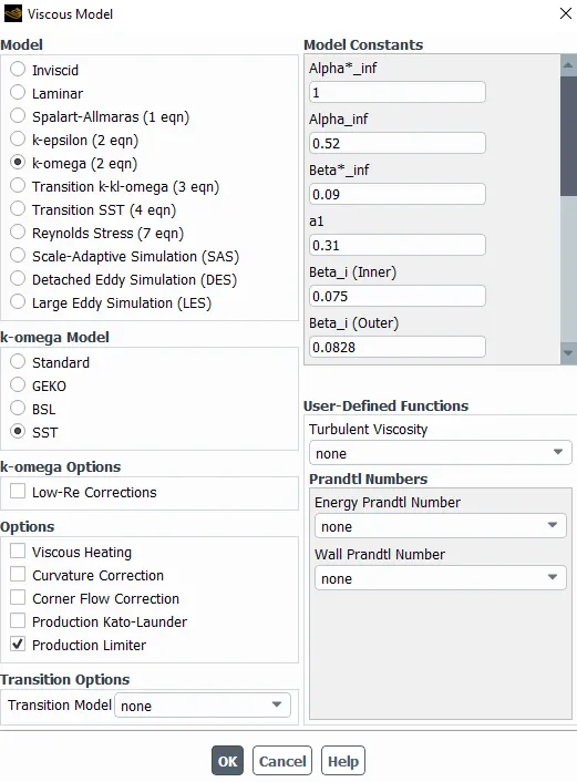
here we are going to go for K-Omega SST model for Use Y+ < 1 for the transition prediction and heat transfer calculations. or Use Y+ < 10 for SST model (omega based models in general) as mentioned in the guide article of understanding Y+.

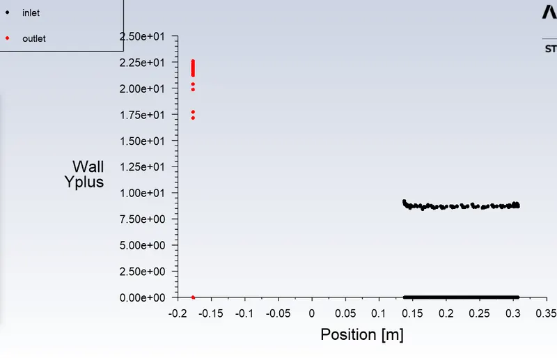
The Y+ is 25 for a given Y+ value of 5.

So here we have selected :

1. K-epsilon turbulence model with standard near-wall treatment for

2. K- epsilon turbulence with Scalable near-wall treatment

3. K-Omega SST turbulancee model.

Here's why we selected the above:

1. For very high Reynolds number flows, where boundary layer becomes very thin and effects of it are not important.
2. For high Mach number flow, consequently, Reynolds number is also very high, again boundary layer is thin and results are dependent on shock wave resolution rather than boundary layer resolution.
3. Flow with no separation, and still, you are trying with Y+ of order 1 or less. In this case, you are increasing round-off error. This will be counterproductive as you are not understanding flow physics.

In the Hybrid wall functions article, you will see that now new hybrid wall function is applicable for all Y+ values. But keep in mind that these hybrid wall functions are designed for SA and K-Omega type models (SST included). However, K-Epsilon type models are designed for wall functions i.e. Y+ >30. But with one equation treatment for K-Epsilon models, you can integrate them to viscous sub-layer. In this case, K-Epsilon-type models require Y+<0.2. This is also known as an enhanced wall treatment.

Now based on the above article you can see that, the strict value of Y+ < 2 for the SST model and Y+ < 1 for the SA model is now not a must. So keeping Y+ up to 10 will give you the same results as of mesh with Y+ ~ 1.

Also, note that for transition modeling (laminar to turbulence transition) you need mesh with Y+ < 1 everywhere along with the requirement of fine mesh in a stream-wise direction.

Based on the above discussion I would like to give you some guidelines / best practices:

1. Keep Y+ below 10 for viscous dominate flows with separation.
2. Use Y+ < 1 for the transition prediction and heat transfer calculations.
3. Use Y+ < 10 for SST model (omega based models in general)
4. Use the K-Epsilon model with scalable wall functions (default option in the new version of Fluent). It will keep the Y+ above 11.06 so that it does not suffer the limitation of old standard wall functions. Moreover, now you can carry the successive refinement of mesh, which was not possible with standard WFs.

Now I would like to give you some results which I ran on Ahmed Body with Hexa Mesh with Y+ < 1 and Y+ ~ 10.

Calculate the wall/surface heat transfer coefficient on the internal solid surface & show the velocity & temperature contours in appropriate areas.

this is how we calculated the wall and surface heat transfer coefficient on the internal solid surface. We exported the CDAT file to CFD-Post from fluent and observed the calculated and achieved results for the above.

Wall Heat Transfer coefficient.

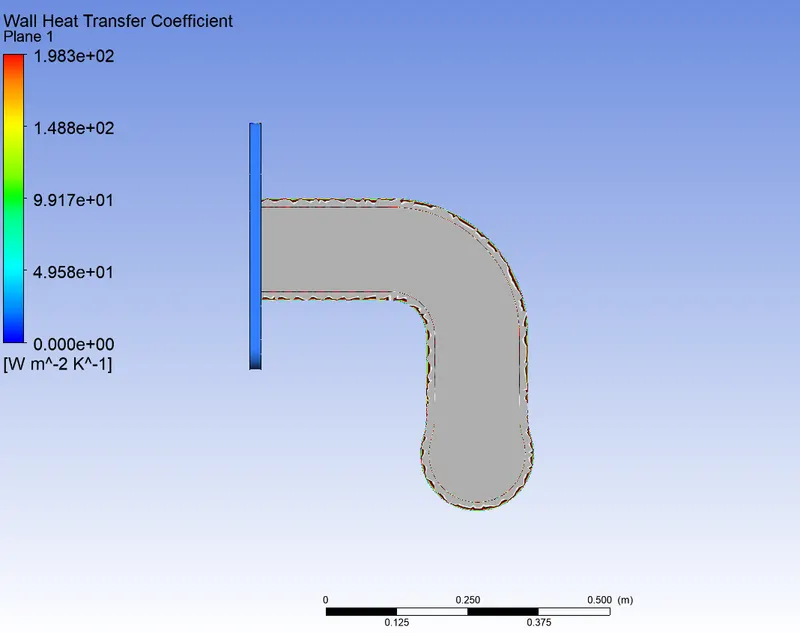
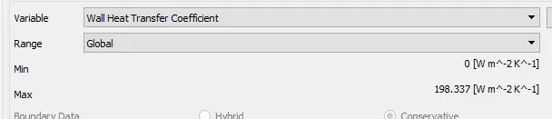
198.337 Wm-2K^-1

Surface Heat Transfer coefficient:

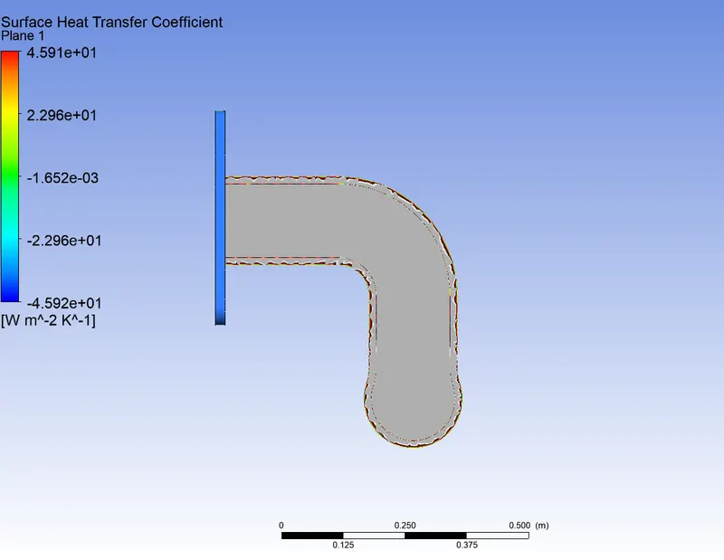
45.914 Wm^-2 K^-1

How would you verify if the HTC predictions from the simulations are right? On what factors does the accuracy of the prediction depend on?

The comparison between the CFD-predicted HTCs and the correlation-predicted HTCs. The multivariable linear correlation tends to overpredict heat transfer at lower values of HTC but underpredict spray cooling at higher values. The exponential correlation shows similar trends as well. The predictions from the single variable linear correlation are more accurate than the other two at lower values of HTC, then the predictions become oscillating between overpredicting and underpredicting at larger HTC values.

Overall, the multivariable linear correlation is the best fit among all three correlations in terms of accuracy. Besides, it only involves two basic mathematic operations, i.e. multiplication and addition. Such features should allow fast prediction, thereby enabling real-time casting control. However, the other two correlations can still be considered as potential candidates. With careful calibration of the combined single variable, the more sophisticated mathematic operations in these two correlations can better reveal the intertwined nature between the casting operating parameters.

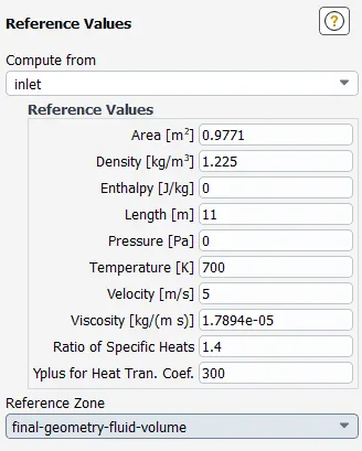
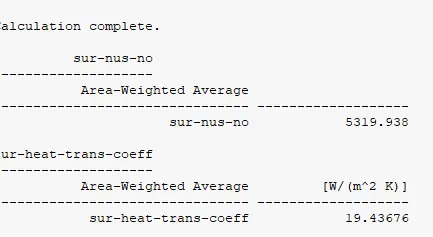
This is what what we got the numerical solutions from fluent and then we go to analytical solutions to validate our result and for that have nusslet number, reynolds number and prandlt relations this where we can determine the analytical solutions.

The Dittus-Boelter equation (for turbulent flow) is an Expilicit functions for calculating the Nusselt number. It is easy to solve but is less accurate when there is a large temperature difference across the fluid. It is tailored to smooth tubes, so use for rough tubes (most commercial applications) is cautioned. The Dittus-Boelter equation is:

and we got Nu = 2334 h = 32.14 W/m^2 K as Analytical solutions and Nu = 5319.9 h = 19.W/m^2 K.

Reference:

Conjugate Heat Transfer Analysis | Analysis Types | SimScale

Conjugate Heat Transfer | COMSOL Blog

Fluid Mechanics 101 - For First Layer calculation.

How to extract the y+ value from fluent ? (researchgate.net)

Understanding Y+ for CFD Simulations (linkedin.com)

Frontiers | Numerical Development of Heat Transfer Coefficient Correlation for Spray Cooling in Continuous Casting | Materials (frontiersin.org)