Week-4 Challenge WOT Condition Part-2

1. comparison between mapped and dynamic models:

Mapped models	Dynamic models
1. Here, the data required for simulating and analysing the model are to entered in the form of a lookup table which will be eventually utilised by the components in the power train.	Dynamic model is more or less similar to machine learning i.e., it updates the behaviour of every component accordingly by gleaning the data from its previous behaviour. It also hands out a concise analysis of data keyed in by us.
2. Simulation time reduces drastically if the lookup table is available.	Here there is no need for any collation of data. It is a real time-based system which operates dynamically depending on the circumstances.
Engine: 3. Mapped engine model represents a holistic behaviour of the engine. Brake torque, mass flow rate of air and fuel and exhaust gas temperatures are recorded using this model.	Dynamic engine model is used to compute the dynamic quantities of the engine such as speed of turbocharger, intake flow rate etc.,
Motor: 4. Mapped motor models are simulated using the parameters such as speed in rpm, heat generated, efficiency for a given speed and torque spectrum.	Here the parameters taken into consideration will be mainly efficiency, torque and rpm for real time analysis of the motor.
Generators: 5. Parameters such as state of charge (SOC), battery current and voltage, state of Health (SOH) will be plugged into the lookup table.	All the parameters in the mapped model will be considered here too.

2.

The three main inputs to Miles Per Gallon block are:

1. Vehicle speed
2. Volume flow rate of fuel
3. Battery power

These are depicted accordingly in the picture below.

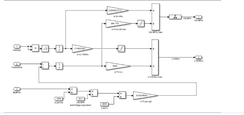
Since the fuel flow rate is in m^3/s we have to convert the volume into gallons to get MPG and the corresponding calculations are explained below:

W.K.T 1 U.S gallon = 3.785 litres

Also 1 m^3 = 1000 litres.

Therefore, 1 gallon = 0.003785 m^3

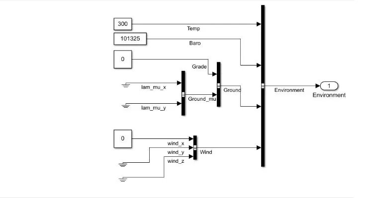
3. The WOT drive cycle is simulated by keeping wind velocity and gradeability zero. The following results were yielded.

The cycle was run for about 40 seconds.

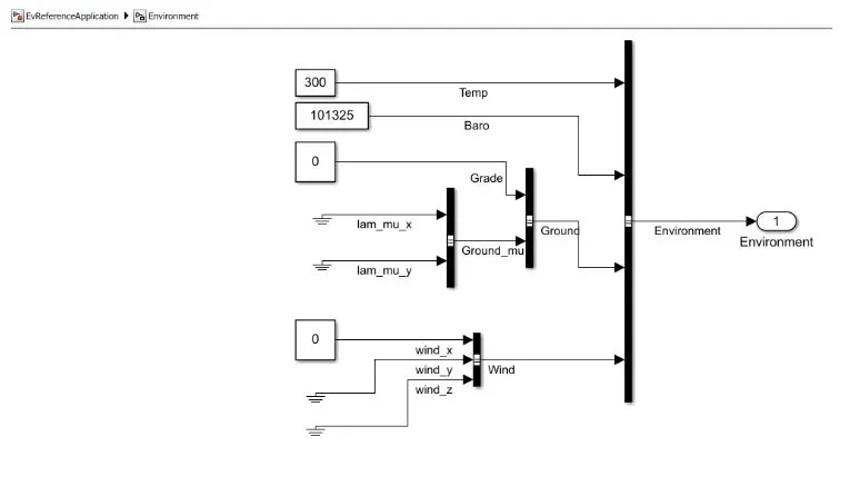
Here the wind velocity and the gradeability are set to zero.

The simulated reults are as follows:

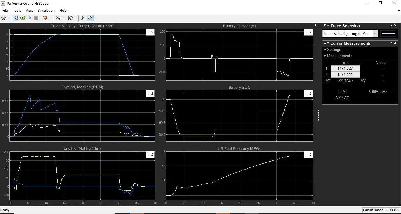
Explanation of the above graphs:

1. Trace velocity target vs Actual:

It is apparent that the vehicle velocity has met target velocity after a while. The desired velocity (yellow line) is at 60 mph and the HEV motor (blue line) takes around 13 seconds to reach that speed.

2. Battery current plot:

This graph gives the undulations in power produced by the battery through current in amperes.

3. Engine speed vs motor speed:

This graph gives the information about speed of the engine and motor in rpm. Clearly the engine speed is higher than the motor speed.

4. SOC graph:

This plot tells us how the battery was drained from the moment HEV started running.

5. Engine torque vs motor torque (N-m):

The motor torque soars way higher than the engine torque at almost 175 N-m compared to that of engine which reaches its pinnacle at 50 N-m. The slump of both the torques denotes braking of the vehicle.

6. MPGe plot:

This is the plot which gives us the information about fuel efficiency of the vehicle.

On changing the grade and wind velocity in the WOT drive cycle, the following results were obtained:

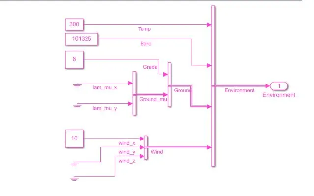
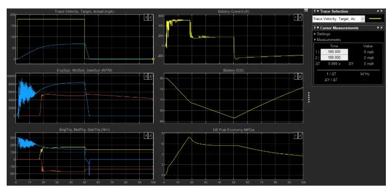
The explanation of the graphs remains the same as above. By changing the wind velocity to 10 mph in x-direction (against the vehicle direction of motion) and increasing the gradeability to 8% we can see massive changes in Battery SOC and MPG.

From MPGe plot, we can say that the fuel consumption has shot up drastically (MPGe reduced to almost 7 MPGe from a peak of 13 MPGe) and Soc plot tells us that SOC drops hard due to the added resistance of wind velocity and gradeability.

Also, the motor is required to generate a lot of torque to overcome the added resistances. So, the motor torque also has skyrocketed.

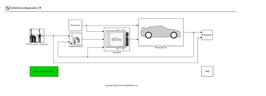
4. Keeping the HEV parameters same and simulating the model, the following results were simulated for zero gradeability and zero wind velocity.

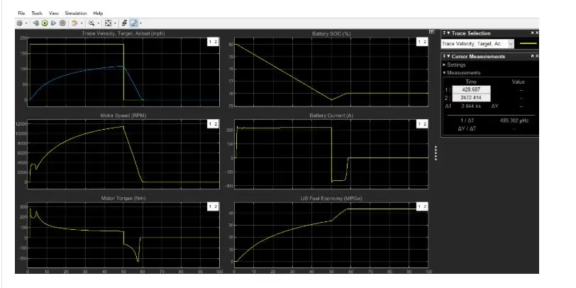
The simulated results of the EV reference application for same parameters as that of HEV are as follows:

Conclusion:

1. EV fails to achieve the desired speed within speculated time with the available propulsion power whereas a hybrid vehicle’s speed easily climbs up to the target speed in a matter of seconds.
2. Battery current of a EV remains immutable until a braking point is reached. So it kind of delivers a constant power throughout. This is not the case in HEV where there is waxing and waning of current.
3. In EV, SOC drops down linearly and reaches a constant value after a threshold.
4. Motor speed gradually builds up gradually in EV whereas in HEV, motor speed is highly arbitrary with time as it works in conjunction with ICE.
5. Motor torque is higher in HEV compared to EV’s.
6. When it comes to MPGe, EV’s are way out of reach to HEV’s which soars at around 44 MPGe while HEV’s can hardly reach 13 MPGe.