Week 4.1 - Solving second order ODEs

SOLVING SECOND ORDER ODEs

AIM

To write a program that solves the following ODE. This ODE represents the equation of motion of a simple pendulum with damping.

In the above equation,
g = gravity in m/s2, 9.81m/s2.
l = length of the pendulum in m, 1 meter.
m = mass of the ball in kg, 1 kg.
b = damping coefficient, 0.05.

EXPLANATION OF THEORY

Ordinary differentional equations (ODEs) is differentional equation containing one or more function of one independent variable and the derivatives of those functions.

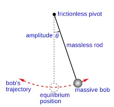
Simple pendulum is an idealized mathematical model of a pendulum,there is a weight on the end of a massless cord suspended from a horizontal rod without friction,It will swiing back and forth at a constant amplitute when we will give an initial push.

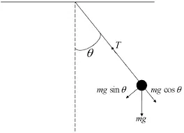
The weight suspended is form which point is known as point of suspension and weight acts vertically downwards and the tension acts vertically upwards, if we will apply smaller external force weight will start oscillating because of equilibrium position.

FUNCTION CODE

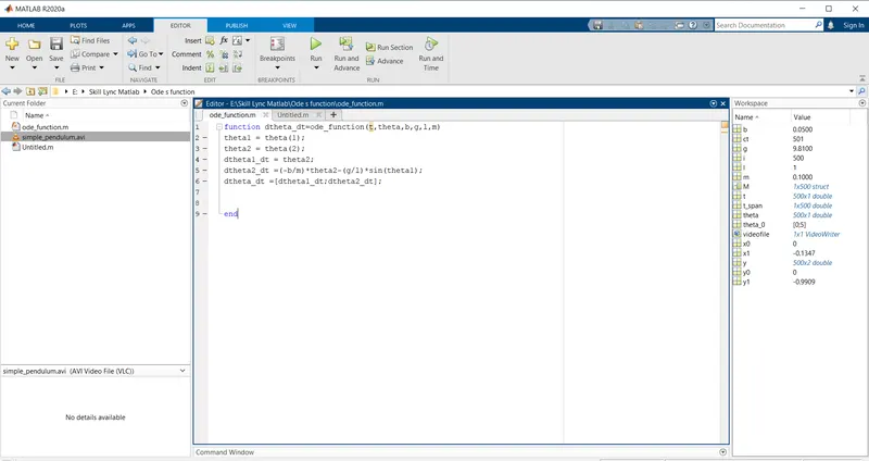
We have to save this function file with same name which we created in coding and save the file in same path where we save the main code.

function dtheta_dt=ode_function(t,theta,b,g,l,m)
theta1 = theta(1);
theta2 = theta(2);
dtheta1_dt = theta2;
dtheta2_dt =(-b/m)*theta2-(g/l)*sin(theta1);
dtheta_dt =[dtheta1_dt;dtheta2_dt];
 
 
end

MAIN CODE

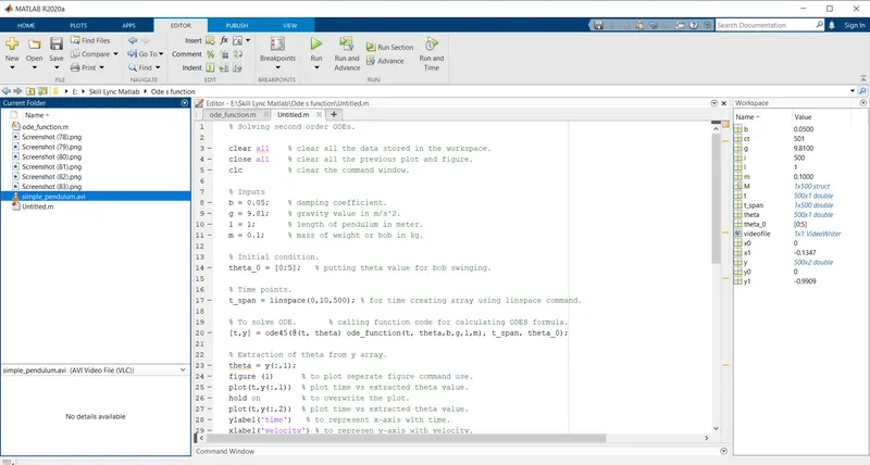
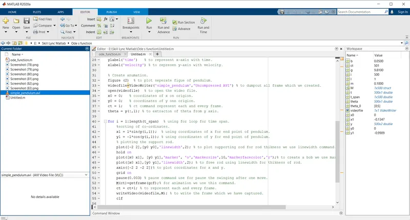
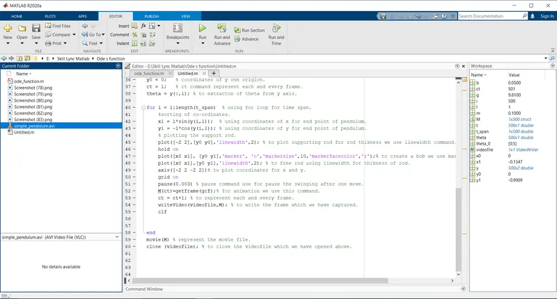
% Solving second order ODEs.
 
clear all    % clear all the data stored in the workspace.
close all    % clear all the previous plot and figure.
clc          % clear the command window.
 
% Inputs
b = 0.05;    % damping coefficient.
g = 9.81;    % gravity value in m/s^2.
l = 1;       % length of penfulum in meter.
m = 0.1;     % mass of weight or bob in kg.
 
% Initial condition.
theta_0 = [0;5];   % putting theta value for bob swinging.
 
% Time points.     
t_span = linspace(0,10,500); % for time creating array using linspace command.
 
% To solve ODE.       % calling function code for calculating ODES formula.
[t,y] = ode45(@(t, theta) ode_function(t, theta,b,g,l,m), t_span, theta_0);
 
% Extraction of theta from y array.
theta = y(:,1);  
figure (1)      % to plot seperate figure command use.
plot(t,y(:,1))  % plot time vs extracted theta value.
hold on         % to overwrite the plot.
plot(t,y(:,2))  % plot time vs extracted theta value.
ylabel('time')   % to represent x-axis with time.
xlabel('velocity') % to represen y-axis with velocity.
 
% Create anumation.
figure (2)  % to plot seperate figue of pendulum.
videofile=VideoWriter('simple_pendulum','Uncompressed AVI') % to dumpout all frame which we created.
open(videofile)  % to open the video file.
x0 = 0;   % coordinates of x on origion.
y0 = 0;   % coordinates of y onn origion.
ct = 1;   % ct command represent each and every frame.
theta = y(:,1); % to extracton of theta from y axis.
 
for i = 1:length(t_span)  % using for loop for time span.
    %sorting of co-ordinates.
    x1 = l*sin(y(i,1));  % using coordinates of x for end point of pendulum.
    y1 = -l*cos(y(i,1)); % using coordinates of y for end point of pendulum.
    % plotting the support rod.
    plot([-2 2],[y0 y0],'linewidth',2); % to plot supporting rod for rod thikness we use linewidth command.
    hold on
    plot([x0 x1], [y0 y1],'marker', 'o','markersize',10,'markerfacecolor','r');% to create a bob we use marker command size of 10. 
    plot([x0 x1],[y0 y1],'linewidth',2); % to free rod using linewidth for thikness of rod.
    axis([-2 2 -2 2])% to plot coordinates for x and y.
    grid on
    pause(0.003) % pause command use for pause the swinging after one move.
    M(ct)=getframe(gcf);% for animation we use this command.
    ct = ct+1; % to represent each and every frame.
    writeVideo(videofile,M); % to write the frame which we have captured.
    clf 
 
          
end
movie(M) % represent the movie file.
close (videofile); % to close the videofile which we have opened above.

EXPLANATION OF THE CODE

⦁ Clear all – clear all the data stored in the workspace.
⦁ Close all – clear all the previous plot and figure.
⦁ Clc – clear the command window.
⦁ First we have given input according to the question linke value or bore, gravity force, length of pendulum, mass of the bob or weight.
⦁ After that put initial condition for bob movement.
⦁ then use linspace command for creating array.
⦁ Call the function code which we have written in function code.
⦁ Extracted the theta from y array.
⦁ Plot figure 1 for separate figure then plot the time vs extracted y array. And then use hold command to overwrite the plot. And also give xlabel and ylabel command to represent the axises.
⦁ Using for loop for creating the pendulum at multiple degree.
⦁ Creating coordinates for origin and end point of the bob.
⦁ After that plot figure 2 separately for pendulum and give all required data.
⦁ Then make an animation video with all required data.
⦁ Then close the code and save the function and main code in same path and run the code to get the result.

RESULT IN GRAPH

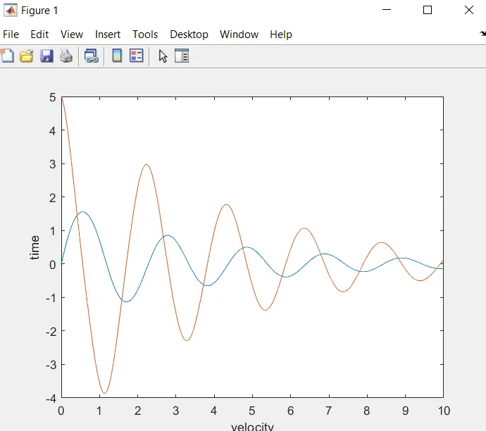
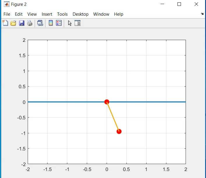
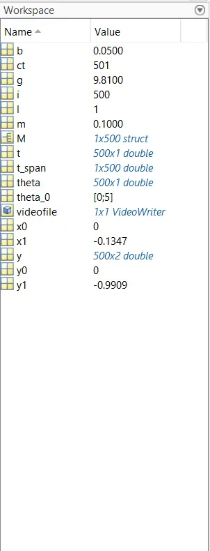
RESULT IN WORKSPACE

ERRORS AND SOLUTION

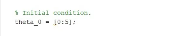
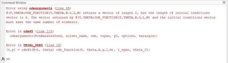
ERROR 1

SOLUTION 1

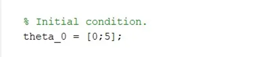
To fix that problem we have used semi colon at the place of colon.

ERROR 2

SOLUTION 2

To fix that problem we have use as the rate (@) symbol.

ERROR 3

SOLUTION 3

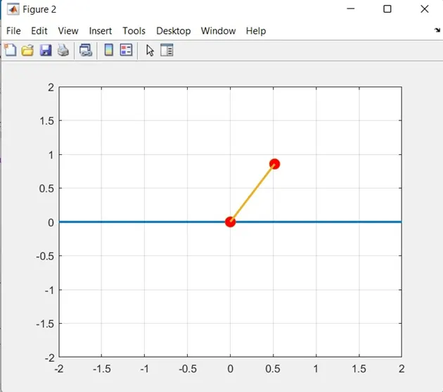
To fix that problem we have used (-) symbol in coordinates of y axis.

YOU TUBE LINK OF ANIMATION

https://youtu.be/9eUd7QsOZYs