Objective:
- To write a program that solves the second order
ordinary differential equation for motion of simple pendulum with damping.
- Simulate the motion of the pendulum using the
generated results.
The equation given is as follows:

Where,
b = damping coefficient
m = mass of the bob in kg
g = gravity in m/s2
L = length of the pendulum in meters
1.
Solving the problem:
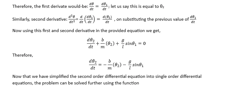
To solve this problem, the function “ode45” in MATLAB is
utilized. Since the function can only solve a single order differential
equation, the provided second order differential equation is broken down into
series of first order differential equations.
Let us assume that θ = θ1
Code:
clc
clear all
close all
%%intializing the values
b = 0.05;
g = 9.81;
m = 1;
l = 1;
%%creating a function that will simplify the second order differential equation into series of single order differential equations
function [derivative] = derive(t,theta,b,g,m,l)
%assigning the first value of the solution array theta to theta1 and second value of the solution array theta to theta2
theta1 = theta(1);
theta2 = theta(2);
%since we considered that the first derivate of theta1 is theta2
first_derivative = theta2;
%%therefore substituting the value of first derivative of theta1 in the equation we get
second_derivate = -(b/m)*theta2 - (g/l)*sin(theta1);
%%returning the second order equation as two first order equations columnwise
derivative = [first_derivative;second_derivate];
end
%initial condition
%%considering angular displacement is zero and angular velocity is 3
%%rad/sec at t=0 secs
theta_initial = [0;3];
%for a motion of 20 seconds
t_span = linspace(0,20,200); %taking 200 values of time between 0 and 20 secs
%solving the second order differential equation using function ode45
[t, results] = ode45(@(t, theta) derive(t,theta,b,g,m,l),t_span,theta_initial);
%%plotting the generated results
figure(1); %for plotting the displacement of the bob w.r.t to time
displacement = results(:,1); %since the first column of the solution includes the values of displacement
plot(t,displacement,'Color','r');
xlabel('time in secs');
ylabel('Displacement in meters');
figure(2); %For plotting the angular velocity w.r.t to time
velocity = results(:,2); %since the second column of the solution includes the values of velocity
plot(t,velocity);
xlabel('time in secs');
ylabel('Angular velocity in m/s');
%plotting displacement and anglular velocity vs time in the same graph
figure(3);
plot(t,displacement,t,velocity);
legend('Displacement (m)','angular velocity (m/s)');
%Simulating the pendulum motion
%first fixing the pedulum
figure(4);
plot([0 0],'b-','LineWidth',3,'color', 'b');
%finding the coordinates of the bob and the pendulum rod with respect to
%displacement angle
x = l*sin(displacement);
y = -l*cos(displacement);
%%creating a loop that will plot the coordinates during the total time span
for i = 1:length(t)
%creating the fixed base of the pedulum
plot([-2 2],[0 0],'b-','LineWidth',5);
hold on;
%to plot the pendulum rod with a line width 2 and a color black
plot([0 x(i)],[0 y(i)],'linewidth',2,'color','k');
hold on;
%to plot the bob as a red marker of size 10
plot(x(i),y(i),'ro','markersize',10,'MarkerFaceColor','r');
title(sprintf('Simple pendulum motion at t=%f secs',t(i)));
%fixing the axis limits
xlim([-l l]);
ylim([-2 1]);
%captures each frame and stores it in a structure M
M(i)=getframe;
clf reset; %clears the figure after every iteration
end
%create a movie file for the structure M
videofile = VideoWriter("Simulation of a pedulum.avi","Uncompressed AVI");
open(videofile);
writeVideo(videofile,M)
close(videofile)
Errors occurred: 
The error was returned due to incorrect syntax used while calling the function, error was fixed was replacing square brackets '[]' with parentheses '()'
Output:
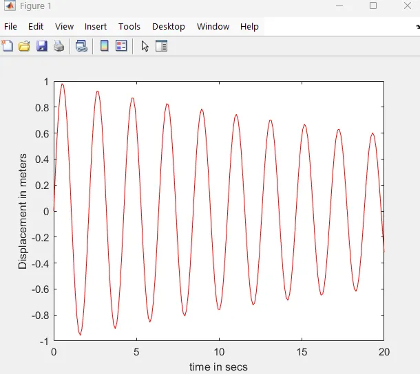
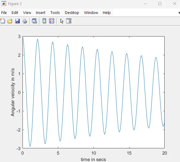
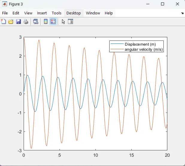
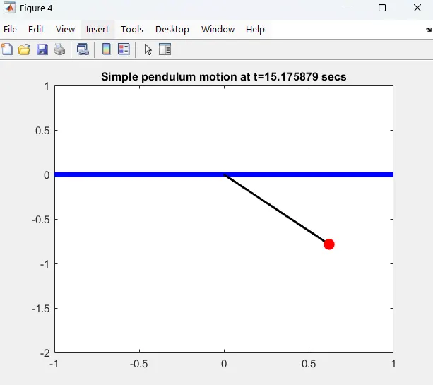
The movie for the simulation of the pedulum can be accessed using google link: https://drive.google.com/file/d/1k4Eku6TyvYLbGHVzBm5-j7LRQ-q6QTl6/view?usp=drive_link
Conclusion: Any higher order differential equations can be solved using different ode functions in Matlab considering the equation is first broken down into simpler single order differential equations.