Week 4.1 - Solving second order ODEs
SOLVING 2ND ORDER ODE
AIM: To write a program that solve the ODE which represents the equation of motion of a simple pendulum with damping.
THEORY:
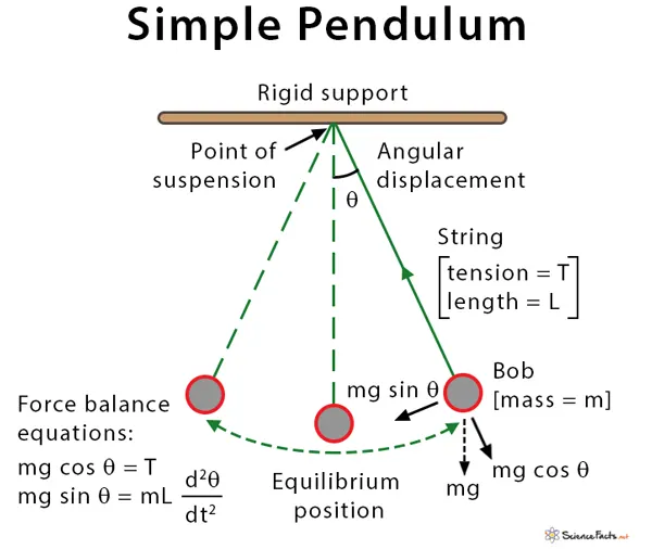
WHAT IS SIMPLE PENDULUM ?
- A simple pendulum is a mechanical arrangement that demonstrate periodic motion.
- It comprises a small bob of mass (m) suspended by thin string secured to a platform at its upper end of length (L).
- And is mainly driven by gravitational force (g).
WHAT IS ODE45 ?
ODE45 is a sophisticated built in MATLAB function that gives accurate solutions. This is the solver to be tried for most problems.
Sove nonstiff defferential equations, it integrate the differential equations from initial time to end time with initial conditions.
EQUATION OF THE MOTION:
`(d^2theta)/dt^2 + (b/m)*(d theta)/dt + (g/l)*sin theta = 0`
b - Damping coefficient (it is a material propety that indicates whether a material will bounce back or return energy to a system )
m - Mass of the bob
l - length of the string
g - acceleration due to gravity
PROCEDURE:
Before starting the program we should break down the second order into first order equation.
BREAKING THE EQUATION:
`(d^2theta)/dt^2 + (b/m)*(d theta)/dt + g/l *sin theta = 0`
considering `theta = theta1`
and by replacing it we get
`(d theta )/dt = (d theta 1)/dt = theta2`------------1
and now `(d^2 theta)/dt^2 = (d^2 theta 1)/dt^2 = (d/dt)*(d theta1 )/dt = (d theta2)/dt`------------2
by combaining equation 1 and 2 we get
`(d theta 2)/dt + b/m*theta2 + g/l* sin theta = 0`
`(d theta 2)/dt = -b/m theta2 - g/l sin theta`
considering it as a matrix we get
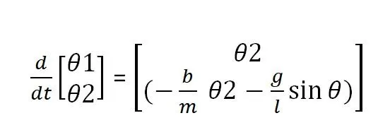
Now we have converted the 2nd order equation to 1st order.
Now with the above equation we need to create a seperate funtion to solve this problem
start the function with the function command and give name to it
function[dtheta_dt] = ode_func(t,theta,b,g,l,m)------[here t and theta can be defined in next main program]
and now we can define theta 1 and theta 2 as above:
theta1 = theta(1);
theta2 = theta(2);
dtheta1_dt = theta2;-----------1st ode
dtheta2_dt = -(b/m)*theta2-(g/l)*sin(theta1);----------2nd ode
dtheta_dt = [dtheta1_dt;dtheta2_dt];---------combaining both ode
CODE FOR FUNCTION :
function[dtheta_dt] = ode_func(~,theta,b,g,l,m)
theta1 = theta(1);
theta2 = theta(2);
dtheta1_dt = theta2;
dtheta2_dt = -(b/m)*theta2-(g/l)*sin(theta1);
dtheta_dt = [dtheta1_dt;dtheta2_dt];

end
Next we can write the code for solving the above equation ploting the graph between angular velocity and displacement with respect to time and to create a video of simle pendulum.
Start the program with clear, close all, clc.
Now we can define the inputs to solve the above conditions, those are:
Damping coefficient b = 0.01
Acceleration due to gravity g = 9.81
Length of the string l = 1
Mass of the bob m = 0.1
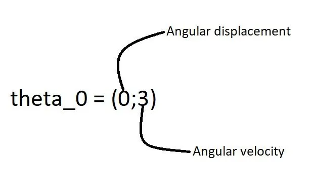
and defining the initial condition i.e, angular displacement and angular velocity:
theta_0 = (0;3)
and defining the time limit
t_span = linspace(0,20,600)
Now to solve the ode we are going to use imbuilt command ode45 to solve the equation
common ode45 command
[TOUT,YOUT] = ode45(ODEFUN,TSPAN,Y0)
[t,results] = ode45(@(t,theta) ode_func(t,theta,b,g,l,m),t_span,theta_0); --------- {here we use the function thet we created before which will use the t_span and theta_0 to solve the equation.}
Now to plot displcement and velocity wrt time:
figure(1)
Plot(t,results(:,1))-------plotting displcement
hold on
plot(t,results(:,2))-------plotting velocity
PLOTTING BOTH DISPLACEMENT AND VELOCITY IN SAME PLOT:
[t,results] = ode45(@(t,theta) ode_func(t,theta,b,g,l,m),t_span,theta_0); --------- {here we use the function thet we created before which will use the t_span and theta_0 to solve the equation.}
Now to plot displcement and velocity wrt time:
figure(1)
Plot(t,results(:,1))-------plotting displcement
hold on
plot(t,results(:,2))-------plotting velocity
PLOTTING THE PENDULUM:
Next making a video of swinging pendulum.
start with figure(2) and stating a for loop to execute the function for several time before starting it begin with counter [ct = 1;]
What is counter ?
It is a variable that simply increment or decrement by a specific step value in every iterationof loop.
The length of the for loop should be the displacement that we calculated above
for i = 1:length(results(:,1))
And now we are going to define the points where the pendulum going to move
so,
x0 = 0;
y0 = 0;
x0 and y0 are the starting points of the plot.
x1 = l*sin(results(i,1));
y1 = l*cos(results(i,1));
x1 and y1 are the ending points of the plot.
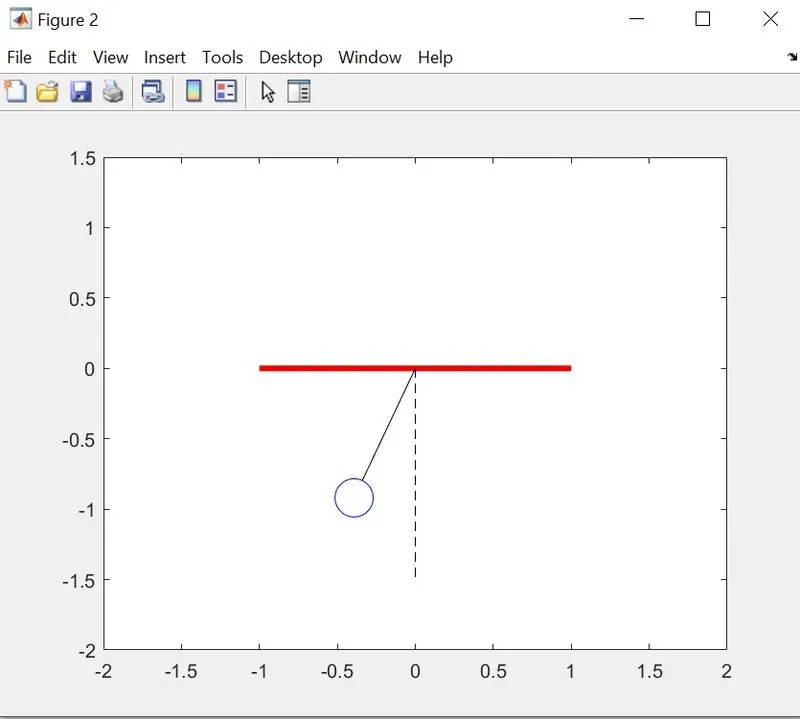
And now we are going to plot the moving pendulum
First plotting the rigid support of the pendulum
plot([-1 1],[0 0], 'linewidth',3,'color','r')
And giving the hold on command to plot the other parts of the pendulum
Next plotting the string of the pendulum
plot ([x0 x1],[y0 y1],'color','black')
Now we are going to plot the bob
plot(x1,y1,'o','MarkerSize',20,'MarkerFaceColor','auto','color','b')
And defining the axis ([-2 2 -2 1.5])
and finally plotting the center axis for the pendulum
plot ([0 0],[0 -1.5],'LineStyle','--','color','black')
And giving hold off
Now we have given plot command to plot thependulum and now we are going to create a movie before that we need to capture the frame i.e capturing the plot to make a movie
F(ct) = getframe(gcf)
and increasing the counter at the end of the loop
ct = ct+1
end
After ending the loop we are going to create the video file
movie(F)
videofile = VideoWriter('pendulum.avi')
open(videofile)
writeVideo(videofile,F)
close(videofile)
Finish the proggram and run it.
CODE:
clear
close all
clc
b = 0.01;
g = 9.81;
l = 1;
m = 0.1;
%initial condition
theta_0 = [0,3];

%time points
t_span = linspace(0,20,600);

%solve ODE

[t,results] = ode45(@(t,theta) ode_func(t,theta,b,g,l,m),t_span,theta_0);
figure(1)
plot(t,results(:,1))
hold on
plot(t,results(:,2))
ylabel('plot')
xlabel('time')
legend('displacement','velosity')
title('ploting displacement,velosity wrt time')

figure(2)
ct = 1;
for i = 1:length(results(:,1))
    x0 = 0;
    y0 = 0;

    x1 = l*sin(results(i,1));
    y1 = -l*cos(results(i,1));

    plot([-1 1],[0 0],'linewidth',3,'Color','r')%plotting support for the pendulum
    hold on
    plot([x0 x1],[y0 y1],'color','black')%plotting string for suspention
    hold on
    plot (x1,y1,'o','MarkerSize',20,'MarkerFaceColor','auto' ,'Color','b')%plotting the bob
    axis([-2 2 -2 1.5])
    plot([0 0],[0 -1.5],'LineStyle','--','Color','black')%plotting equilibrium line

    hold off
    F(ct) = getframe(gcf);

    ct = ct+1;
end

% creating a video file
movie(F)
videofile = VideoWriter('pendulum.avi');
open(videofile)
writeVideo(videofile,F)
close(videofile)
DISPLACEMENT VELOCITY GRAPH:
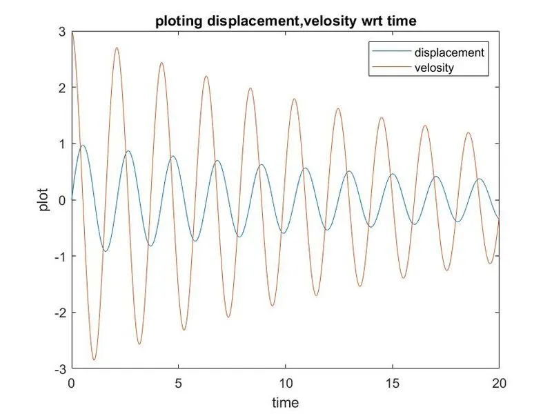
LINK FOR VIDEO:
https://youtu.be/iTPkI-LFDaE
ERROR FACED DURING THE PROGGRAM:
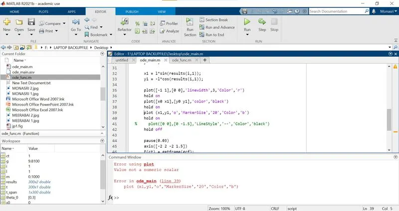
The error was rectified by changing the '20' in plot command markersize into 20.