Week 4.1 - Solving second order ODEs

Objective-

To write a program that solves the following ODE. This ODE represents the equation of motion of a simple pendulum with damping.

Damping –

In physical systems, damping is the loss of energy of an oscillating system by dissipation. Damping is an influence within or upon an oscillatory system that has the effect of reducing or preventing its oscillation. Examples of damping include viscous damping in a fluid (see viscous drag), surface friction, radiation, resistance in electronic oscillators, and absorption and scattering of light in optical oscillators. Damping not based on energy loss can be important in other oscillating systems such as those that occur in biological systems and bikes.

Damping Ratio –

The damping ratio is a dimensionless measure describing how oscillations in a system decay after a disturbance. Many systems exhibit oscillatory behavior when they are disturbed from their position of static equilibrium.

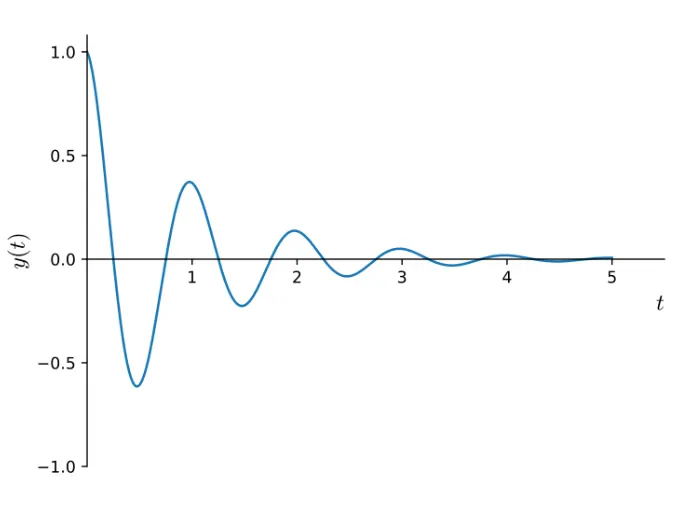
Damped sine wave –

A damped sine wave or damped sinusoid is a sinusoidal function whose amplitude approaches zero as time increases. It corresponds to the underdamped case of damped second-order systems, or underdamped second-order differential equations.

Introduction to using ode45 in MATLAB –

MATLAB’s standard solver for ordinary differential equations (ODEs) is the function ode45. This function implements a Runge-Kutta method with a variable time step for efficient computation. ode45 is designed to handle the following general problem:

dx/dt = f(t, x), x(t0) = x0, ….. Eq.(1)

where

t is the independent variable,

x is a vector of dependent variables to be found and

f(t, x) is a function of t and x.

The mathematical problem is specified when the vector of functions on the right-hand side of Eq. (1), f(t, x), is set and the initial conditions, x = x0 at time t0 are given.

MATLAB SCRIPT SYNTAX

MAIN CODE -

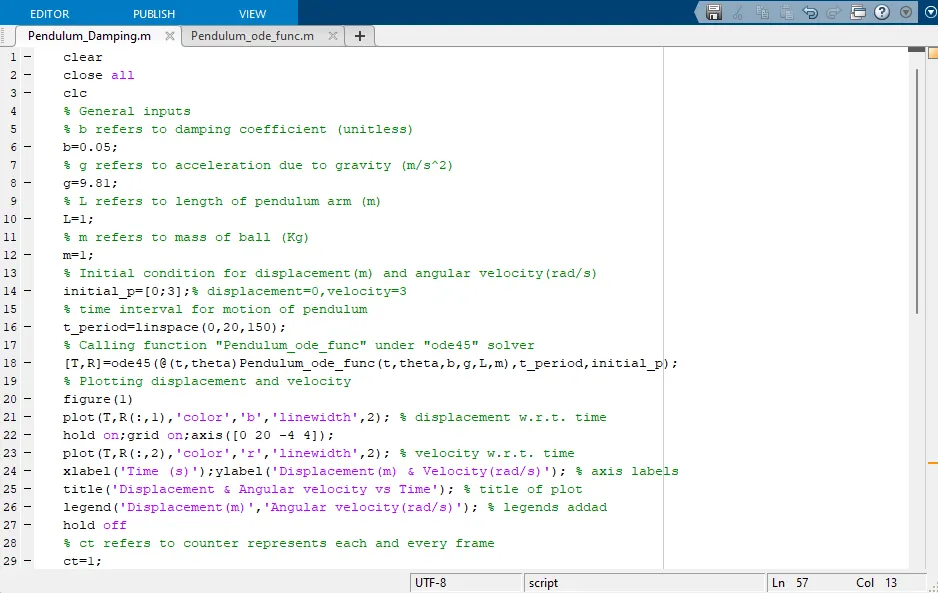
clear
close all
clc
% General inputs
% b refers to damping coefficient (unitless)
b=0.05;
% g refers to acceleration due to gravity (m/s^2)
g=9.81;
% L refers to length of pendulum arm (m)
L=1;
% m refers to mass of ball (Kg)
m=1;
% Initial condition for displacement(m) and angular velocity(rad/s)
initial_p=[0;3];% displacement=0,velocity=3
% time interval for motion of pendulum
t_period=linspace(0,20,150);
% Calling function "Pendulum_ode_func" under "ode45" solver
[T,R]=ode45(@(t,theta)Pendulum_ode_func(t,theta,b,g,L,m),t_period,initial_p);
% Plotting displacement and velocity
figure(1)
plot(T,R(:,1),'color','b','linewidth',2); % displacement w.r.t. time
hold on;grid on;axis([0 20 -4 4]);
plot(T,R(:,2),'color','r','linewidth',2); % velocity w.r.t. time
xlabel('Time (s)');ylabel('Displacement(m) & Velocity(rad/s)'); % axis labels
title('Displacement & Angular velocity vs Time'); % title of plot
legend('Displacement(m)','Angular velocity(rad/s)'); % legends addad
hold off
% ct refers to counter represents each and every frame
ct=1;
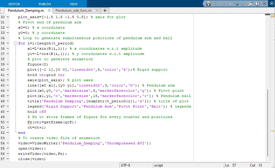
plot_axis=[-1.5 1.5 -1.5 0.5]; % axis for plot
% Pivot end of pendulum arm
x0=0; % x coordinate
y0=0; % y coordinate
% Loop to generate simultaneous positions of pendulum arm and ball
for i=1:length(t_period)
    x1=L*sin(R(i,1)); % x coordinates w.r.t amplitude
    y1=-L*cos(R(i,1)); % y coordinates w.r.t amplitude
    % plot to generate animation
    figure(2)
    plot([-1 1],[0 0],'linewidth',5,'color','k');% Rigid support
    hold on;grid on;
    axis(plot_axis); % plot axes
    line([x0 x1],[y0 y1],'linewidth',3,'color','b'); % Pendulum arm
    plot(x0,y0,'o','markersize',5,'markerfacecolor','g'); % Pivot point
    plot(x1,y1,'o','markersize',15,'markerfacecolor','r'); % Pendulum ball
    title('Pendulum Damping',[num2str(t_period(i)),'s']); % title of plot
    legend('Rigid Support','Pendulum Arm','Pivot Point','Ball'); % legends
    hold off
    % Pn to store frames of figure for every counter and positions
    Pn(ct)=getframe(gcf);
    ct=ct+1;
end
% To create video file of animation
video=VideoWriter('Pendulum_Damping','Uncompressed AVI');
open(video);
writeVideo(video,Pn);
close(video)

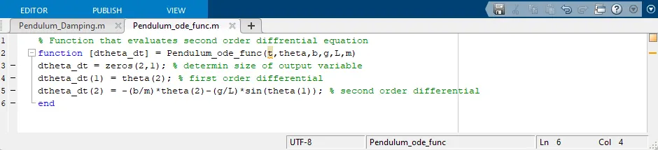
FUNCTION CODE –

% Function that evaluates second order diffrential equation
function [dtheta_dt] = Pendulum_ode_func(t,theta,b,g,L,m)
dtheta_dt = zeros(2,1); % determin size of output variable
dtheta_dt(1) = theta(2); % first order differential
dtheta_dt(2) = -(b/m)*theta(2)-(g/L)*sin(theta(1)); % second order differential
end

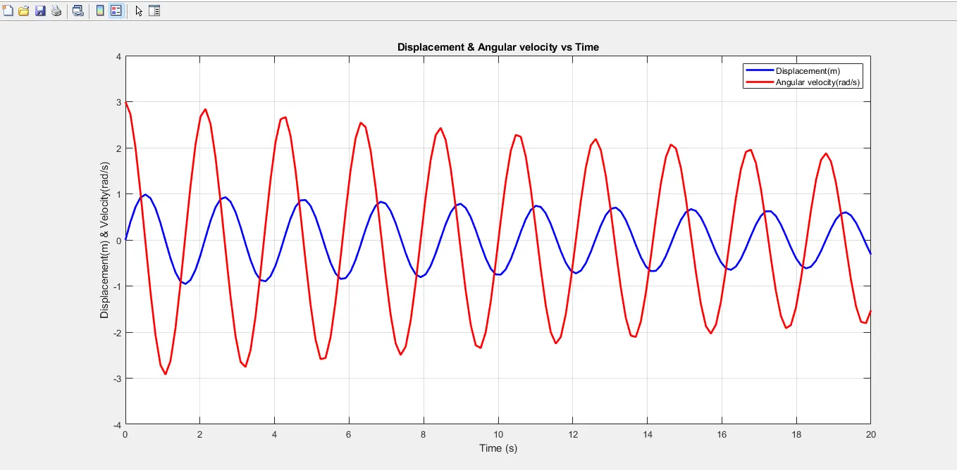
OUTPUT PLOT –

ANIMATION VIDEO –

Google drive link :

Link - https://drive.google.com/file/d/1T0eLvrCgqGxKvsvPJljcCYupNz8pPrXW/view?usp=drive_link

Video - Pendulum_Damping.avi

SNAPSHOTS –

==================================================================