Challenge

Week 4.1 - Solving second order ODEs

NNayan Nag15 Dec 2022

Aim:
1. Create code for the equation.

2. Create plot according to the equation.

3. a.Create vedio file and Simulate the motion between 0-20 sec, for angular displacement=0,angular velocity=3 rad/sec at time t=0.
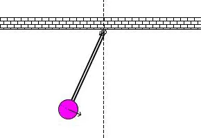
Your animation does not have to look exactly like this and here is the logic.

b. For each value in time
c. Create an image that represents the position of the pendulum
d. You can assume the length of the string and the size of the ball
e. Use the marker command to create a sphere
f. One end of the pendulum is fixed
g. The other end moves according to the solution of the ODE you had solved.
h. If you are using using Matlab, use the movie command create an animation
4. Submit a report that has the following content:

i. Step wise explanation of your code.
ii. Errors faced while programming.
ii. How have you overcome those errors.
Screenshots showing errors thrown in command window.
Objective :
1. write a codescript and function file to run this ODE function.
2. Create plot as per the output of the solution.
3. Create movie or animation of the motion between 0-20 sec, for angular displacement=0,angular velocity=3 rad/sec at time t=0.
4. Upload the vedio on youtube and Drop the youtube link.

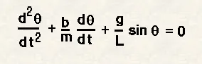
Governing Equation:

Body of the project:

Function file :

function [dtheta_dt] = ode_func(t, theta, b,g,l, m)

theta1 = theta(1);

theta2 = theta(2);

dtheta1_dt = theta(2);

dtheta2_dt=-(b/m)*theta2-(g/l)*sin(theta1);

dtheta_dt = [dtheta1_dt; dtheta2_dt];

end

Main script:

close all

clear all

clc

%PARAMETERS

b=0.05;

g=9.81;

m=0.1;

l=1;

%Initial condition

theta_0 =[0; 5];

% time points

t_span = linspace(0,10,500);

% Solve ODE

[t, results] = ode45(@(t, theta) ode_func(t,theta,b,g,l,m), t_span,theta_0);

plot(t, results(:,1))

hold on

plot(t,results(:,2))

xlabel ('Time in sec')

ylabel ('Angular Velocity')

legend ('Time in Sec', 'Angular Velocity')

title 'ANGULAR VELOCITY VS TIME GRAPH'

amplitude = results(:,1)

grid on

%For Animation

%counter represent each and every frame

ct=1;

for i = 1:length(amplitude);

angle = amplitude(i)

%PIVOT POINT CO-ORDINATE

x0 =0; y0 =0;

x1 = l*sin(angle);

y1 = -l*cos(angle);

plot([-1,1], [0,0], 'linewidth',10,'Color','green')

axis([-2, 2,-0.6, 2])

hold on

% String

plot([x0,x1],[y0,y1],'linewidth',2,'color','blue')

% Bob tied at free end of string

plot(x1,y1,'marker','o','markersize',20,'markerfacecolor','red')

hold off

% Adjustment of axes of plot

axis([-1,1,-2,0])

pause(0.05)

grid on

% Storing each plot as a frame in an array M

M(ct) = getframe(gcf);

ct = ct+1;

end

movie(M);

Videofile = VideoWriter('SIMPLE PENDULUMii.avi');

open(Videofile)

writeVideo(Videofile,M)

close(Videofile)

Explaination:

Clear all is used to clear previous variables, values, size arrays from the workspace

Close all is used to close all the previous program.

Clc is used to clear all the values from the command window.

Initial condition is Adding the inputs , variables in the input- b,g,m & l.

where, b is the damping co-efficient,

g is the gravitationalforce,

m is the mass of the ball,

l is the length of the string.

for getting the plot 'ANGULAR VELOCITY' VS 'TIME' graph - need points which makes the curve.

there is two first order ODE. One is for velocity and another one is for displacement.

so, getting the initial condition we need the value of theta which is actually nothing but the displacement;

So, here taking theta as written below,

theta_0 =[0; 5];

initially I am taking the DISPLACEMENT as '0' and the final VELOCITY as '5'.

As per the ODE rule we have to integrate the ODE system to obtain a solution for which we have to define the value of time 't'.

So,

Taking time as an array with 500 values, which is written below,

t_span = linspace(0,10,500);

then using the ODE45 command,

[t, results] = ode45(@(t, theta) ode_func(t,theta,b,g,l,m), t_span, theta_0);

Here, we are using the ode45 command which can be provided in the form of anonymous function.

if i explain it with a equation then it will be written as,

function_handle =@(input_arguments)function_definition

where,

function handle is [t, result]

input_argument is @(t, theta)

function_ definitio is ode_func(t,theta,b,g,l,m) which is created in the new page script of matlab.

t_span is the array which is required to integrate the intial time period to final time period,

theta_0 is the initial position of the pendulam.

for plotting,plot command is used

plot(t, results(:,1))

hold on

plot(t,results(:,2))

for labeling the x and y axis, label command is used.

xlabel ('Time in sec')

ylabel ('Angular Velocity')

for pointing the name of different colour curve data "legend' command is used

legend ('Time in Sec', 'Angular Velocity')

for giving the title of the graph title command is used.

title 'ANGULAR VELOCITY VS TIME GRAPH'

'grid' command is used for displaying the grid line in the graph.

grid on

Explaination the function_file:

code script is below,

function [dtheta_dt] = ode_func(t, theta, b,g,l, m)

theta1 = theta(1);

theta2 = theta(2);

dtheta1_dt = theta(2);

dtheta2_dt=-(b/m)*theta2-(g/l)*sin(theta1);

dtheta_dt = [dtheta1_dt; dtheta2_dt];

end

Explaination:

Here the second order ODE has been converted into first order ODE by representing theta as theta1 and (dθ/dt) as theta2 then (d^2θ/dt) will become (dθ1/dt).

theta1 is the angular velocity and theta2 is angular displacement respectively.

Here, we have represented the two ODE as,

dtheta1_dt = theta2
dtheta2_dt = -(b/m)*theta2 - (g/l)*sin(theta1) and then solution vector is created dtheta_dt.

Then the function is imported to the main matlab program.

For Creating The Animation file:

amplitude = results(:,1)

The reason I am taking the amplitude so that i can save the each and every matrix of resulsts(:,1) in the workspace.

next, apply for loop to get the iteration,

i = 1:length(amplitude);

where,

angle = amplitude(i)

takiing initial value of x0 point and y0 point is,

x0 =0; y0 =0;

for the forward and backward motion or displacement of the pendulam can be equate by those equation,

x1 = l*sin(angle);

y1 = -l*cos(angle);

For plotting the fixed horizontal plane where string is attached

plot([-1,1], [0,0], 'linewidth',10,'Color','green')

For fixing the axis , 'axis' command is used

axis([-2, 2,-0.6, 2])

for getting the plane visible in the Graph,'hold on' command is used.

hold on

For plotting string

plot([x0,x1],[y0,y1],'linewidth',2,'color','blue')

For plotting Bob tied at free end of string

plot(x1,y1,'marker','o','markersize',20,'markerfacecolor','red')

For stopping the repetitive visible plots os string and the bob while moving forward and backward 'hold off'

command is used

hold off

Adjustment of axes of plot

axis([-1,1,-2,0]) is used

for getting the gridline in the animation 'grid on' command is used

grid on

for creating the animation

initialy, taking the counter value as 'ct=1' and after first iteration it will go to second iteration and it will runs automatically untill the last itteration.

here, i am taking the variable 'M' as an array and for getting the iteration of 500 times .
i want an increment of 'ct' as each and everytime after forloop get executes. thats why i am writing the counter value as

'ct =ct+1'

after that i am ending the for loops so that code get executed and complete the iteration as per the equation inside the for loop and get
different positioned plot which is used to make the video.

For getting the visualise the animation for particular time the command will be written as

pause(' write required time')

i.e ,

pause(0.05)

For making movie I am using movie(M) command.
for naming the Videofile = VideoWriter('forward_kinematics.avi'); command is used
for opening the video file open(videofile) command is used.
to write the video 'writeVideo(Videofile,M)' command is used.
for closing the videofile 'close(Videofile)' command is used.

after running the whole code, Matlab succesfully created a vedio by using the plot.

Note: I am attaching the youtube link -https://youtu.be/jjzHdQ9eK_M

Conclusion:

From that challenge we can understand how to apply the concept of ODE in Matlab and plot the graph of 'ANGULAR VELOCITY' VS 'TIME'.
We learned to apply the code to create plot of different positions of the pendulam and by the help of these plots we can make a vediofile by the name of 'SIMPLE PENDULAM'.

ERROR FACED AND RECOVERY:

Error and Reason :

The reason for the error is mostly spelling mistakes, missing of parenthese , wrong execution of the command i.e while giving the input of the command bracket() or coma , missing.

Most Fatal Error was graph is not plot properly i.e somtimes horrizontal line and String is not showing, But bob is showing in the graph , also Simple Harmonic Motion of PENDULUM was not showing.

While making the animation file, animation could not be created due to the mistakes in command or spelling mistake of the command.

Recovery:

1.By debugging the code step by step those missing parenthese, brackets and the checking the spelling mistakes of the commands ractified and solved.

2.By discussing with the technical support team and implementing the suggestions in the code the animation and plot created successfully.

3. Checking the command sequence and correcting the commands and inputs the code is recovered successfully

Note: This code runs successfully after 8 times of execution.

Week 4.1 - Solving second order ODEs

Ship work like this
in your own course.

Talk to a career counsellor

Ship work like thisin your own course.

Talk to a career counsellor

Ship work like this
in your own course.