Week 4.1 - Solving second order ODEs

Aim:

To write a program that solves the ODE representing the equation of motion of a simple pendulum with damping.

`(d^2(theta))/dt^2+(b/m)(d(theta))/dt+(g/L)sin(theta)=0`

Here,

g = gravity in m/s2,

L = length of the pendulum in m,

m = mass of the ball in kg,

b=damping coefficient.

Input Data:

Length(L) = 1metre

Mass(m)=1 kg,

Damping Coefficient (b)=0.05.

Gravity (g)=9.81 m/s2

Angular Displacement`(theta)` = 0 radians @ time t=0 sec

Angular Velocity`((d(theta))/dt)` = 3 rad/sec @ time t=0 sec

Time range = 0 to 20 sec

Matlab Code With Comments:

Maincode:

clear all %Clears the workspace
close all %Closes all the plots
clc  % Clears command window

%Inputs
b=0.05;
g=9.81;
l=1;
m=1;

%initial condition at time t=0 sec
theta_0 = [0;3];

%time span
t_span = linspace(0,20,1000);


%Using matlab ODE solver to solve the system of equation
[t,results] = ode45(@(t,theta) ode_func(t,theta,b,g,l,m),t_span,theta_0);
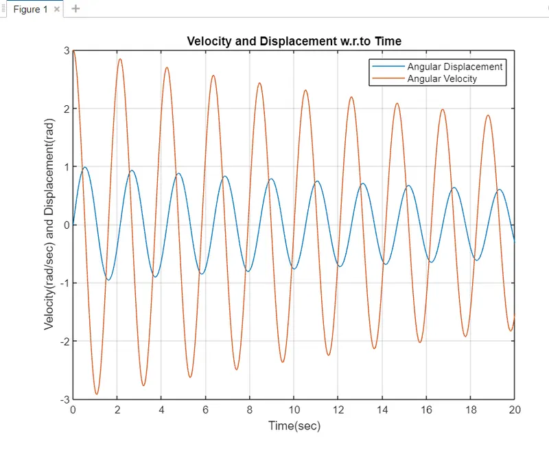
%Figure 1 plots shows how velocity and dispacement are changing w.r.to time.
figure(1)
plot(t,results(:,1))
hold on
plot(t,results(:,2))
ylabel("Velocity(rad/sec) and Displacement(rad)")
xlabel("Time(sec)")
title('Velocity and Displacement w.r.to Time')
legend('Angular Displacement','Angular Velocity')
grid on

%Figure 2 helps to creates the animation video of simple pendulum by capturing each
%frame
figure(2)
ct=1;
for i = 1: length(t_span)
    x_0=0;
    y_0=0;
    x_1=l*sin(results(i,1));
    y_1 =-l*cos(results(i,1));
    plot([-1.5 1.5],[0 0],"linewidth",3,"Color","k")
    hold on
    plot([x_0 x_1],[y_0 y_1],"linewidth",3,"Color","b")
    plot(x_1,y_1,".","MarkerSize",50,"Color","r")
    axis([-1.5 1.5 -1.5 1.5])
    M(ct) = getframe(gcf)
    hold off
    ct=ct+1;
end
%Each frame is combined to form a movie
movie(M)
videofile=VideoWriter('simple pendulum.avi','Uncompressed AVI');
open(videofile)
writeVideo(videofile,M)
close(videofile)

Function Code:

%Defining the function
function [dtheta_dt] = ode_func(t,theta,b,g,l,m)
    %Indexing operation 
    theta1 = theta(1);
    theta2 = theta(2);
    %substituting the values in 2 first order ode
    dtheta1_dt = theta2;
    dtheta2_dt = -(b/m)*theta2 -(g/l)*sin(theta1);
    dtheta_dt=[dtheta1_dt;dtheta2_dt]; %solution vectors
end

Explanation of Coding Logic:

• clear all clears the workspace. close all closes the plots. clc clears command window.
• Provide the input data b,g,l,m,time span, angular dispacement and angular velocity at time(t) = 0 sec.

Syntax Explanation of ODE45:

[tSol , ySol] = ode45(@(t,y) fName(t,y) , [t0 , tEnd] ,y0)

tSol , ySol : Solution vectors; matlab returs ySol for each time tSol

fName :Fuction that returns dy = F(t,y)

t0,y0 : Initial conditions at time t=0sec

tEnd: Final value until which the solution is desired.

• Using ODE45 solver to obtain the results(angular displacement , angular velocity) with respect to time.
• In figure 1, plotting the graph between angular velocity vs time and angular displacement vs time.Format the plot with title,legend,xlabel,ylabel,grid on.
• In figure 2 for each value in time, the position of pendulum is captured using get current frame command. These frames are then stitched together to form a movie.
• Intially the counter(ct) = 1.For each frame the counter(ct) will be updated.
• The position of pendulum is calculated using trignometric relations.The angular displacement`(theta)` is obtained from results of ode solver.
• Use plot command to plot the positions x0,x1,y0,y1.

• movie command combines all the frame captured by variable 'M' and makes a movie.

• VideoWriter is used to create uncompressed AVI file and it is stored in a variable name called videofile.

• The video file is opened, the movie is written into video file and then closed.

Animatio video link:

https://youtu.be/38X15JEqppc

Graph:

Error Faced:

In the command movie, the first letter is written in upper case. so it throws a error.

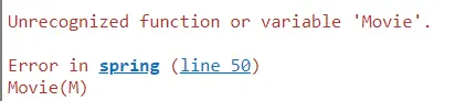
To overcome this error, the "m" should be in lowercase.

Result:

Thus by using Matlab ode45 solver the motion of simple pendulum is simulated.