Week 4.1: Project - Steady state simulation of flow over a throttle body

Steady-state simulation of flow over a throttle body

Objectives:

• Perform a Steady State simulation of flow over a throttle body and post-process the results.

Throttle Body:

• The throttle body is a flow controlling valve used in IC engines to control the intake air and in process industries in the form of a butterfly valve. In IC engines it is placed to either increase or decrease the power and in process industries, it is used for the transportation of fluid or gases at desired rates.
• The basic principle lies behind achieving desired flow rate by rotating the plate at an optimum angle. 0 deg and 180 deg corresponds to zero and max flow rate respectively.
• They can be operated using either mechanical or electrical actuators.

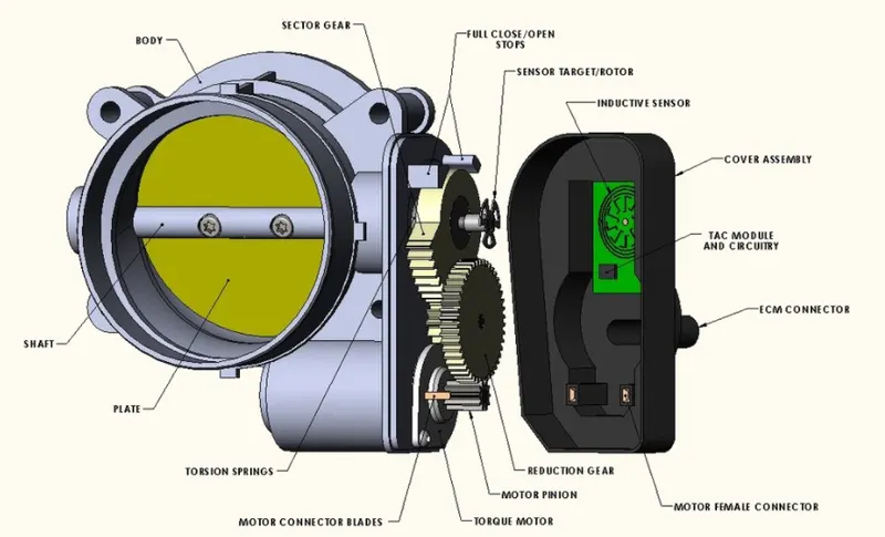
Fig. (a). Throttle Valve

Geometry:

• Figure (b) shows a throttle plate located at the bend parallel to the pipe cross-section when viewed from the front. This indicated that it is positioned at 180 deg. (fully open, max. flow rate)

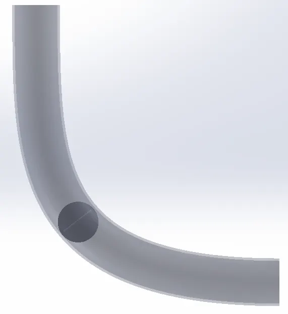
Fig (b). Geometry of simplified throttle body

• Fig (c). shows the triangulated geometry in converge solver and its dimensions along 3 axes.

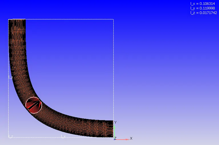
Fig (c). Triangulated Geometry

Case Setup:

Fluid Regime: Air

Simulation Type: Steady State (energy equations are not solved as the temperature is not a subject of interest in this particular study)

Solver: Pressure-Implicit with Splitting of Operators (PISO), Density-based. (Generally used for high speed flows but here it is used as its solution is more robust with respect to this solver)

Turbulence Model: RANS RNG k-ε

Steady State Monitor:

• The minimum number of cycles to be executed is set to 5000. This ensures that the solver does not stop before 5000 cycles even if the solution is converged.
• Monitor Start Delay is set to 5000 cycles as well, this ensures that the convergence criterion is checked only after 5000 cycles.
• The sample size is set to 1000. This indicates the minimum number of consecutive iterations to pass the convergence criterion.

• 

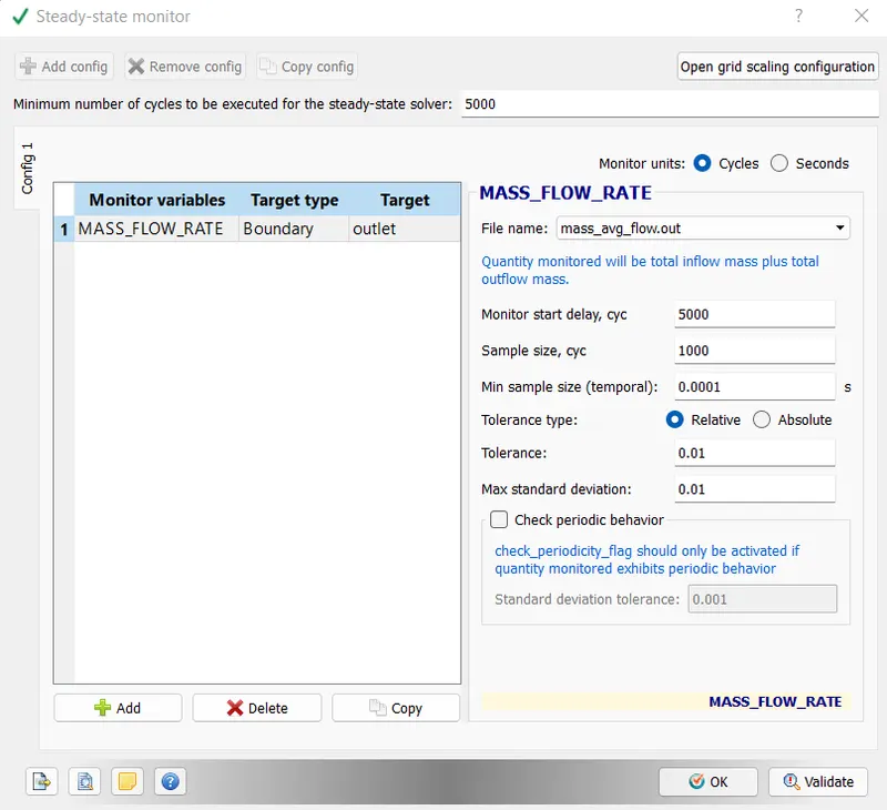
Fig (d). Steady State Monitor setup

Simulation time parameters:

• The maximum number of cycles expected to run even if convergence is not achieved is set to 15000.
• Initial time step is set to 1e-09s while final time step is 1s
• Max. convection and diffusion CFL limits are set to 1.0 and 2.0 respectively. This ensures that the flow is solved without any instability.

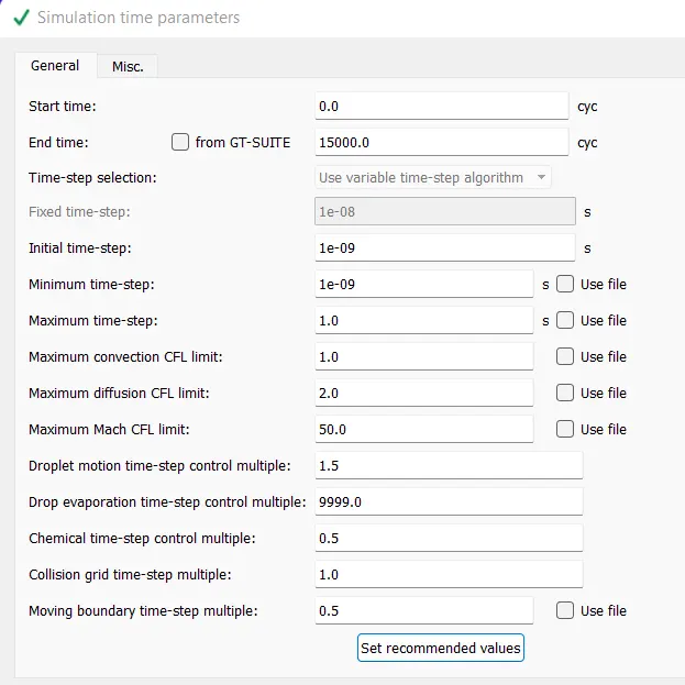
Fig (e). Simulation time parameters

Boundary conditions:

Inlet: Pressure inlet-150000 Pa

Outlet: Pressure outlet-100000 Pa

Throttle Plate: Wall

Elbow Pipe: Wall

Initial conditions: 101325 Pa

Meshing (Discretization):

• 0.002 m along X,Y,Z directions with fixed embedding at the interface between the throttle plate and pipe wall.
• Total no. of cells: 35518

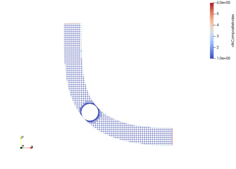
Fig. (f). Cross-sectional view of the mesh

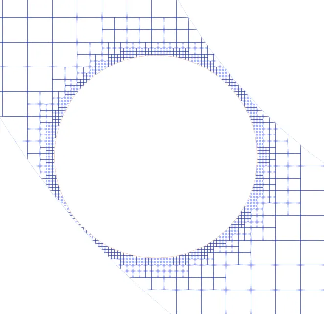
Fig (g). Refinement of grid near throttle plate using fixed embedding technique.

Results:

Velocity Contour: (Click here for detailed contour development)

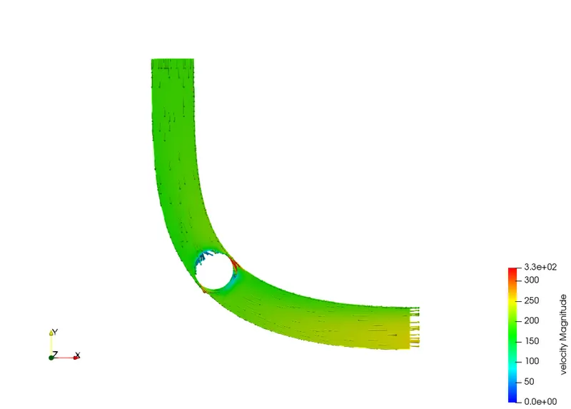
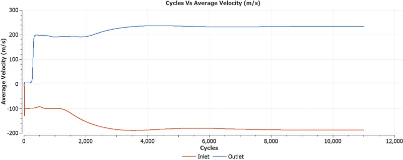
Inference: Velocity at the outlet is 234.34 m/s. However, a peak magnitude of 330m/s is achieved in the interface between the throttle plate and pipe wall.

Pressure contour: (Click here for detailed contour development)

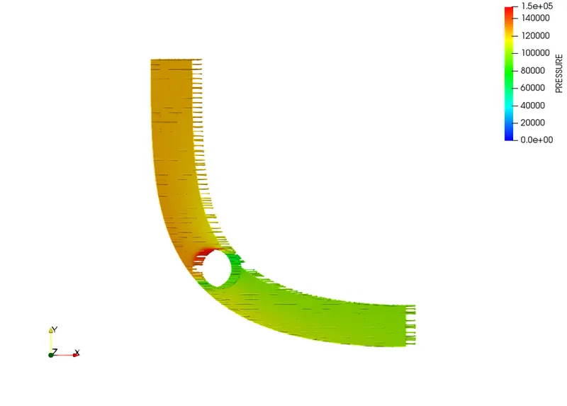
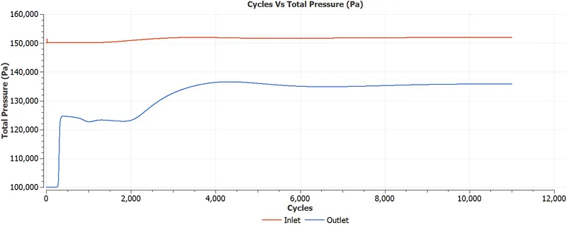
Inference-Total pressure at the inlet is 151850 Pa and at the outlet is 135805 Pa. Peak pressure occurs at the entry face of the throttle plate.

Mass flow rate:

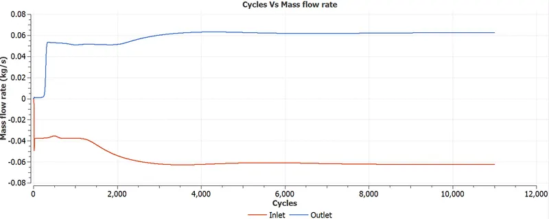
Inference-Both flow rates (inlet and outlet) have converged to the same magnitude which shows that the mass is conserved.

References:

[1] https://www.solerengineering.com/technical