Week 4.1 - Genetic Algorithm

Aim: To find the global maxima for the stalagmite function using genetic algorithm in MATLAB

What is a Genetic Algorithm?

A genetic algorithm (GA) is a method for solving both constrained and unconstrained optimization problems based on a natural
selection process that mimics biological evolution. The algorithm repeatedly modifies a population of individual solutions. At each
step, the genetic algorithm randomly selects individuals from the current population and uses them as parents to produce the
children for the next generation. Over successive generations, the population "evolves" toward an optimal solution.
The genetic algorithm uses three main types of rules at each step to create the next generation from the current population:
Selection rules select the individuals, called parents, that contribute to the population at the next generation.
Crossover rules combine two parents to form children for the next generation.
Mutation rules apply random changes to individual parents to form children.

How does the Genetic Algorithm Work?

The following outline summarizes how the genetic algorithm works:
1. The algorithm begins by creating a random initial population.
2. The algorithm then creates a sequence of new populations. At each step, the algorithm uses the individuals in the current
generation to create the next population. To create the new population, the algorithm performs the following steps:
Scores each member of the current population by computing its fitness value. These values are called raw fitness scores.
Scales the raw fitness scores to convert them into a more usable range of values. These scaled values are called expectation
values.
Selects members, called parents, based on their expectation.
Some of the individuals in the current population that have lower fitness are chosen as elite. These elite individuals are passed
to the next population.
Produces children from the parents. Children are produced either by making random changes to a single parent—mutation—or
by combining the vector entries of a pair of parents—crossover.
Replaces the current population with the children to form the next generation.
3. The algorithm stops when one of the stopping criteria is met.

Genetic Algorithm (ga) Syntax (used in our program):

1. x = ga (@func, nvars), where "func" is the function name and "nvars" is the number of variables.
2. x = ga (@func, nvars, A, B, Aeq, Beq), a set of lower and upper bounds is given so that the solution lies in that range.
3. x = ga (@func, nvars, A, B, Aeq, Beq, lb, ub, nonlcon, IntCon, options), where
A, B = linear inequality constraints
Aeq, Beq = linear equality constraints
lb = lower bound
up = upper bound
nonlcon = non-linear constraints
Intcon = vector of positve integers

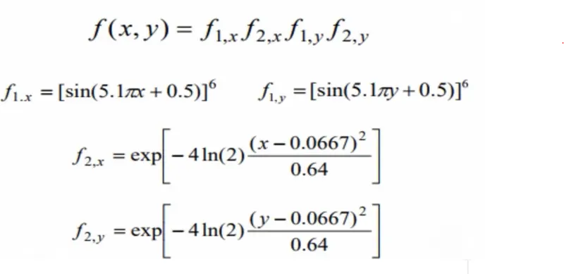
Program for function

function f=stalagmite(input_vector)
x=input_vector(1);
y=input_vector(2);
f1=(sin(5.1*pi*x+0.5))^6;
f2=(sin(5.1*pi*y+0.5))^6;
f3=exp((-4*log(2)*(x-0.0667)^2)/0.64);
f4=exp((-4*log(2)*(y-0.0667)^2)/0.64);
f=-(f1*f2*f3*f4);
end

 matlab coad :-

clear all 
close all
clc

% defining our search space
 n= 150;
x=linspace (0,0.6,150);
y=linspace (0,0.6,150);

% creating a 2 Dimension mesh

[xx, yy]= meshgrid(x,y);

% Evaluating the stalagmite function 

for i= 1:length(xx)
   
    for j=1:length(yy)
        input_vector(1)=xx(i,j);
        input_vector(2)=yy(i,j);
        f(i,j)= stalagmite(input_vector);
    end
end
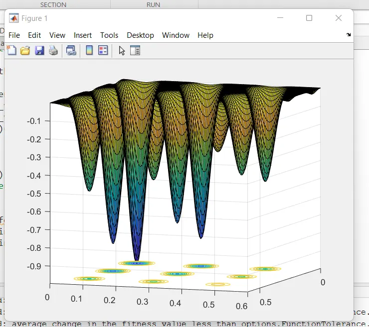
% tip:- (surfc using time xx,yy,-f) usde then the graph shown upper side.

surfc(xx,yy,f);
% shading interp

 for i=1:n
     [inputs,fopt(i)]=ga(@stalagmite,2);
     xopt(i)=inputs (1);
     yopt(i)=inputs(2);
 end
 

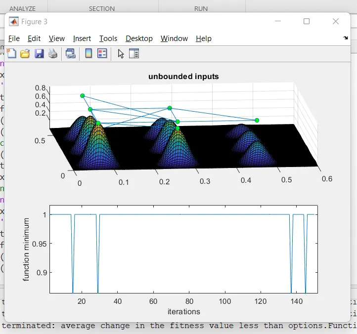
 fig output :-

Matlabe coad :-

clear all
close all 
clc
% Defining our search space 
x =linspace(0,.6,150);
y =linspace(0,.6,150);
num_case=150;
% creating a 2D mesh
[xx,yy]= meshgrid(x,y);
% evaluating the stalagmite function
for i=1:length(xx);
 for j =1:length(yy);
input_vector(1)=xx(i,j);
input_vector(2)=yy(i,j);
f(i,j)= stalagmite(input_vector);
 end
end
tic
 for k = 1:num_case;
 [inp,fval(k)] = ga(@stalagmite,2);
 x_1(k) = inp(1);
 y_1(k) = inp(2);
 end
study1_time=toc
tic
for s = 1:num_case;
 [input,fval(s)]= ga(@stalagmite,2,[],[],[],[],[0,0],[.6,.6]);
 x_2(s)= input(1);
 y_2(s)= input(2);
 
end
study2_time = toc
% 3rd case study increasing ga iterations
options = optimoptions('ga');
options = optimoptions(options,'populationsize',150);
tic
for m = 1:num_case;
 [input,fval(m)]= ga(@stalagmite,2,[],[],[],[],[0,0],[.6,.6],[],[],options);
 x_3(m)= input(1);
 y_3(m)= input(2);
 
end
study3_time = toc
figure (1)
 hold on
 grid on
 surfc(xx,yy,-f)
 shading interp
 title('stalagmite plot')
 xlabel ('X')
 ylabel('Y')
 figure(2)
 subplot(2,1,1)
surfc(xx,yy,-f)
%shading interp
hold on
plot3(x_1,y_1,-fval,'marker','o','markersize',5,'markerfacecolor','g')
title('unbounded inputs')
subplot(2,1,2)
plot(-fval)
xlabel('iterations')
ylabel('function minimum')
% 2nd case study statistical behavior
figure(3)
subplot(2,1,1)
surfc(xx,yy,-f)
%shading interp
hold on
plot3(x_2,y_2,-fval,'marker','o','markersize',5,'markerfacecolor','g')
title('unbounded inputs')
subplot(2,1,2)
plot(-fval)
xlabel('iterations')
ylabel('function minimum')
% 3rd case study increasing ga iterations
figure(4)
subplot(2,1,1)
surfc(xx,yy,-f)
%shading interp
hold on
plot3(x_3,y_3,-fval,'marker','o','markersize',5,'markerfacecolor','g')
title('unbounded inputs')
subplot(2,1,2)
plot(-fval)
xlabel('iterations')
ylabel('function minimum')