Week 4.1 - Genetic Algorithm

Stalagmite Mathematical Model

Aim: To find the Global maxima for the stalagmite function using genetic algorithm in MATLAB

Objectives:

• Write a code in MATLAB to optimise the stalagmite function and find the global maxima of the function.
• Clearly explain the concept of the genetic algorithm in your own words and also explain the syntax for ga in MATLAB in your report.
• Make sure that your code gives the same output, even if it is made to run several times.
• Plot graphs for all 3 studies and for F maximum vs no. of iterations. Title and axes labels are must, legends could be shown if necessary.

Theory:

• Optimisation

Optimisation is a decision making process, it helps to find the best result. Under a set of prioritized criteria or constraints. It is a procedure which is executed iteratively by comparing various solutions till an optimum or a satisfactory solution is found.

• Techniques available to perform optimisation

Deterministic Method: They use specific rules for moving one solution to another. In this technique, the output of the model is fully determined by the parameter values and the initial conditions.

Example: Stress analysis of the component, this is a deterministic approach since the output results(stress values) fully depend on the initial conditions(loading condition) and the parameter values(force acting on the component and material properties).

Stochastic Method: These are gaining popularity due to certain properties which deterministic algorithms do not possess. Stochastic models possess some inherent randomness, it is a probabilistu=ic approach.

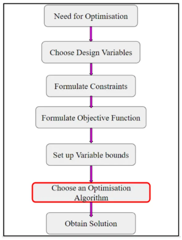
The following is the procedure followed by any optimisation process.

• Genetic Algorithm (GA):

As shown above in the flowchart, we need to choose an optimisation algorithm to perform the optimisation process. Genetic algorithm is one of the optimisation process.

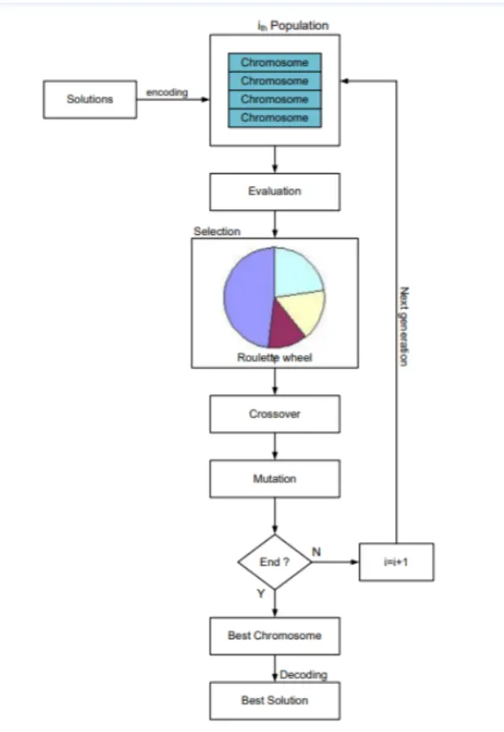
Genetic Algorithm (GA) is a search-based optimisation technique based on the principles of Genetic and Natural Selection. It is frequently used to find optimal or near-optimal solutions.

It is frequently used to solve optimisation problems, in research, and in machine learning.

• How does GA Work?

The following flow chart describes how the genetic algorithm works to find the optimal solution.

Following are the Syntax used for the finding the maximum of the function using genetic algorithm:

x = ga(fun, nvars) finds a local uncontrained minimum, x, to the objective function, fun. nvars is the dimension (number of design variables) of fun.

x = ga(fun,nvars,A,b,Aeq,bed,lb,ub) defines a set of lower and upper bounds on the design variables, x, so that a solution is found in the range lb `<=`x `<=`ub. (Set Aeq=[] and beq=[] if no linear equalities exits.)

x = ga(fun,nvars,A,b,Aeq,beq,lb,ub,nonlcon,options) minimizes with the default optimisation parameters replaced by values in options. (Set nonlcon=[] if no nonlinear costraints exist.) Create options using optimoptions.

where,

fun = Objective function

nvars = Numbers of variables

A =Linear inequality constraints

b = linear inequality constraints

Aeq = Linear equality contraints

beq = Linear equality contraints

lb = Lower bounds

ub = Upper bouds

nonlcon = Nonlinear contraints

options = Optimisation options

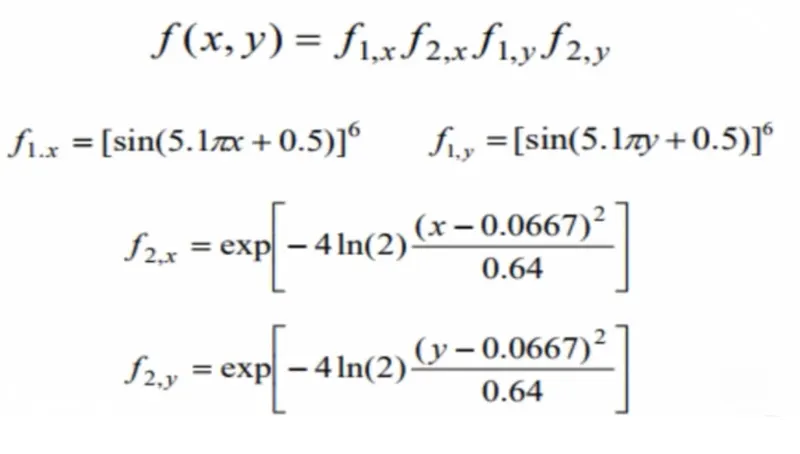
The equation of stalagmite funtion is,

Program for Function

function f=stalagmite(input_vector)

x=input_vector(1);
y=input_vector(2);

f1=(sin(5.1*pi*input_vector(1)+0.5)).^6;
f2=(sin(5.1*pi*input_vector(2)+0.5)).^6;
f3=exp((-4*log(2)*(input_vector(1)-0.0667).^2)/0.64);
f4=exp((-4*log(2)*(input_vector(2)-0.0667).^2)/0.64);

f=-(f1*f2*f3*f4);

end

Program for Global Maxima

clear all
close all
clc


%Defining the search space
x = linspace(0,0.6,150);
y = linspace(0,0.6,150);
num_cases = 50;

%Creating 2Dimensional mesh
[xx yy] = meshgrid(x,y);

tic
for i = 1 : length(xx)
    for j = 1 : length(yy)
        input_vector(1)=xx(i,j);
        input_vector(2)=yy(i,j);
        f(i,j) = stalagmite_function(input_vector);
    end
end

% Study 1 Unbounded
for i = 1:num_cases
    % genetic algorithm for maximization
    [inputs, fopt(i)] = ga(@stalagmite_function,2);
    xopt(i) = inputs(1);
    yopt(i) = inputs(2);
end
study_time1 = toc;
figure(1)
subplot(2,1,1)
hold on
surfc(x,y,-f)
shading interp
title('Unbounded Inputs')
plot3(xopt,yopt,-fopt,'marker','o','markersize',5,'markerfacecolor','r')
subplot(2,1,2)
plot(-fopt)
xlabel('Iterations')
ylabel('Function maximum')

% Study 2 Statistical behaviour within Upper and Lower Bounds
tic
for i = 1:num_cases
    [inputs,fopt(i)]=ga(@stalagmite_function,2,[],[],[],[],[0;0],[0.6;0.6]);
    xopt(i)=inputs(1);
    yopt(i)=inputs(2);
end
study_time2=toc;
figure(2)
subplot(2,1,1)
hold on
surfc(x,y,-f)
shading interp
plot3(xopt,yopt,-fopt,'marker','o','markersize',5,'markerfacecolor','r')
title('Bounded Inputs')
subplot(2,1,2)
plot(-fopt)
xlabel('Iterations')
ylabel('Function maximum')

% Study 3 Increasing the GA Iterations

options = optimoptions('ga')
options = optimoptions(options,'PopulationSize',250);
tic
for i = 1:num_cases
    [inputs,fopt(i)]=ga(@stalagmite_function,2,[],[],[],[],[0.6;0.6],[],[],options);
    xopt(i)=inputs(1);
    yopt(i)=inputs(2);
end
study_time3=toc
subplot(2,1,1)
surfc(x,y,-f)
shading interp
hold on
plot3(xopt,yopt,-fopt,'marker','o','markersize',5,'markerfacecolor','r')
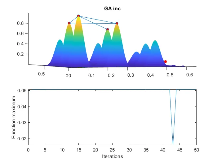
title('GA inc')
subplot(2,1,2)
plot(-fopt)
xlabel('Iterations')
ylabel('Function maximum')

Step by Step Explanation:

1. First, we write a code to define the stalagmite function. Here we break down the formula into 4 terms for convenience
2. Then we write the main code where we define two inputs x and y both of which are one dimensional equally spaced array containing 100 elements. We utilize mesh grid command to create an array of x and y values.
3. Now we use for loop to input value of the 2D array in stalagmite function are obtained. Here we encounter a problem i.e. every time the code is excuted different values for stalagmite function are obtained. This is overcome by introducing another loop into the code. We then input these values into the genetic algorithm. For the genetic algorithm 'ga' function is used
4. 4.To improve our Genetic Algorithm, we under take three cases to optimize the function so that we can accurately find the global maxima of the function. We need to do this because GA randomly takes values and global maxima can change according to that.
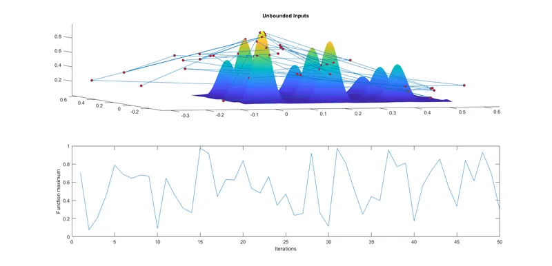
5. In case 1 we evaluate all possible maxima for all the iteration using a loop. We two lot in figure using suplot command. 'surfc' command is used for x vs y graph and for function max vs iteration we use simple 'plot' command. The values in figure (1) are unbounded values.
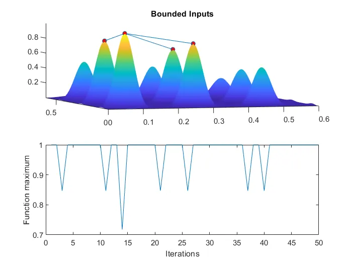
6. Incase 2 we put an upper bound and lower bound on 'ga' function and again plot two plots which we plot during case 1.
7. Incase 3 we increase GA iterations. We do this because in GA after successive iterations, the population "evolves" toward an optimal solution i.e more the number of iterations, more optimal the solution will be. Now we use the same commands to plot the graph and curve.

Output:

Study-1 Unbounded inputs:

Study-2 Bounded inputs:

Study-3 Increasing the GA Iterations: