Week 4.1 - Genetic Algorithm
Aim-
To utilize the concept of genetic algorithm to optimize stalagmite function; finding the global maxima of the function.
Objective-
Studying the optimization of stalagmite function using MATLAB programming to find the global maxima under different optimization setup conditions.
Background-
Mathematical optimization can be defined as the selection of the best possible element or variable criteria out of the possible alternatives that fulfill the given designed criteria and constraints while maximizing or minimizing the given objective function to achieve the best fit.
When plotted, stalagmite and stalactite functions are mathematical functions that display the curve similar to the stalagmite or stalactite with a peak or valley. In the following study, the following set of equations are used to represent a stalagmite function which is further taken into consideration to optimize while determining the global maxima of the function:
F1x = ( sin ( 5.1*pi*x + 0.5 ) ) 6
F1y = ( sin ( 5.1*pi*y + 0.5 ) )6
F2x = exp( -4*log(2)*( ( x-0.0667 )2 )/0.64 )
F2y = exp( -4*log(2)*( ( y-0.0667)2 )/0.64 )
F = (F1x*F2x*F1y*F2y) ; (Objective function to be maximized)
Genetic Algorithm is one of the optimization techniques used to solve tougher NP problems. It is designed following the footsteps of the natural adaptation process to resolve complex and large datasets.
The GA follows the following five phases to evaluate, cross-examine and terminate the unlikely solutions to present an optimum solution for the given objective function:
- Initial population: generating a pool of initial suitable solutions for the problem.
- Fitness function: evaluating the fitness of each possible solution.
- Selection: evaluating the fitness score of the possible solutions, the variables are then further used to generate the next possible solution generation.
- Crossover: the crossover probability determines the next generation of solutions based on the parent solution class. If there is no crossover, then the offspring solutions are the exact copy of the parent solution.
- Mutation: used to prevent premature convergence while maintaining the diversity of the solution generation.
MATLAB genetic algorithm (GA) function syntax:
Below presented are the predefined list of syntax for the GA functions available on MATLAB:
x = ga(fun,nvars)
x = ga(fun,nvars,A,b)
x = ga(fun,nvars,A,b,Aeq,beq)
x = ga(fun,nvars,A,b,Aeq,beq,lb,ub)
x = ga(fun,nvars,A,b,Aeq,beq,lb,ub,nonlcon)
x = ga(fun,nvars,A,b,Aeq,beq,lb,ub,nonlcon,options)
x = ga(fun,nvars,A,b,Aeq,beq,lb,ub,nonlcon,intcon)
x = ga(fun,nvars,A,b,Aeq,beq,lb,ub,nonlcon,intcon,options)
x = ga(problem)
[x,fval] = ga(___)
[x,fval,exitflag,output] = ga(___)
[x,fval,exitflag,output,population,scores] = ga(___)
Methodology-
- The problem is initially defined by defining the input variables along with the upper and lower bound using ‘linspace’ command for ‘x’ and ‘y’ variables.
- A 2D coordinate grid is created using ‘meshgrid’ command for the ‘x’ and ‘y’ variables.
- Two ‘for’ loops are initiated to evaluate the stalagmite function while calling the objective function and assigning the values to the objective function.
- A separate stalagmite function (stalagmite_function) defines the objective function to be maximised.
- Figure (1), a 3D surface plot with contours is generated of the function with various input values using ‘surfc’ command and ‘shading interp’ command for generating interpolating colormap across the surface.
surfc(xx,yy,-f) : ‘-f’ to maximize the function.
- Labelling and title representation are done on a surface plot displaying the function.
- The study is being conducted in three parts: unbounded random input variables sampling, bounded input sampling and bounded input sampling with additional optimization parameters.
- For study 1; standard GA syntax is being used.
A ‘for’ loop is initiated for 50 iterations with the following GA syntax:
[input1,fopt1(i)] = ga(@stalagmite_function,2);
‘input1’ (array of possible solutions) consists of two values (x and y) for the following unbounded random input sampling, whereas ‘fopt1’ (array of objective function’s value) for the corresponding possible solution values.
The GA calls the function ‘stalagmite_function’ while ‘2’ states the number of design variables (x and y).
- ‘input1’ values are then assigned to their respective arrays ‘xopt1’ and ‘yopt1’.
- Figure (2) is generated with two subplots; the first represents the surface plot with a plot of optimum solution of the objective function values, whereas the second plot represents the plot for 50 iterations and their corresponding values function values.
- ‘plot3’ command is used for 3D plotting of the solutions obtained for each possible solution.
- For study 2; i.e. bounded input sampling, the following syntax is being used:
[input2,fopt2(i)] = ga(@stalagmite_function,2, [], [], [], [], [0 0], [0.6 0.6]);
Syntax: x = ga(fun,nvars,A,b,Aeq,beq,lb,ub)
where, ‘A’, ‘b’, ‘Aeq’ and ‘beq’ are linear inequalities, but since there are no additional inequalities for the following problem, they are left as empty array.
- ‘lb’ and ‘ub’ are defined as lower and upper bound, respectively. Since the lower and upper bound for both ‘x’ and ‘y’ variables are ‘0’ and ‘0.6’ respectively, they are assigned in an array of [0 0] and [0.6 0.6].
- Again, a ‘for’ loop is initiated for 50 iterations.
- ‘input2’ represents the possible values of x and y variables giving the solution, which are then assigned to their respective array ‘xopt2’ and ‘yopt2’, while ‘fopt2’ represents the array of objective function values for the corresponding ‘xopt2’ and ‘yopt2’ values.
- Figure (3) is generated with two subplots; the first represents the surface plot with a plot of optimum solution of the objective function values, whereas the second plot represents the plot for 50 iterations and their corresponding values function values.
- For study 3; i.e., bounded input sampling with additional optimization parameters following syntax is being used:
[input3,fopt3(i)] = ga(@stalagmite_function,2, [], [], [], [], [0 0], [0.6 0.6], [], opt);
opt = optimoptions('ga', 'Display', 'iter', 'MaxGenerations', 1000*3, 'PopulationSize', 500, 'FunctionTolerance', 1e-6, 'PlotFcn', @gaplotbestindiv);
Syntax: x = ga(fun,nvars,A,b,Aeq,beq,lb,ub,nonlcon,options)
nonlcon: nonlinear constraints
optimoptions: returns a set of default options for SolverName- ‘ga’
display & iter: iterative display
maxgenerations: maximum no. of iterations (3000)
population size: 500
function tolerance: The algorithm stops if the average relative change in the best fitness function value is less than or equal to FunctionTolerance.
- Figure (4) is generated with two subplots; the first represents the surface plot with a plot of optimum solution of the objective function values, whereas the second plot represents the plot for 50 iterations and their corresponding values function values.
- Further, the final optimized value of optimum design variables and optimum function values are returned, i.e., ‘input3’ and ‘-fopt3’.
Matlab Programming-
Editor window: (main program)
clc
clear all
close all

%   Defining our search space
x = linspace(0,0.6,150);
y = linspace(0,0.6,150);

%   Creating a 2 Dimensional mesh
[xx,yy] = meshgrid(x,y);

%   Evaluating the stalagmite function
for i = 1:length(xx)                                    %   starting two 'for' loops for changing input variables into stalagmite function
    for j = 1:length(yy)
        input_vector(1) = xx(i,j);
        input_vector(2) = yy(i,j);
        f(i,j) = stalagmite_function(input_vector);     %   calling function
    end
end

figure(1)
surfc(xx,yy,-f)                     %   creates 3-D shaded surfaces with contours
shading interp                      %   color shading of surface by interpolating the colormap index
xlabel('X value')                   %   'x' and 'y' axsis labels
ylabel('Y value')
title('Stalagmite Function')        %   title of figure 1


% Study 1: Unbounded/random input sampling: with random values

for i = 1:50                                            %   'for' loop for 50 iterations
    [input1,fopt1(i)] = ga(@stalagmite_function,2);     %   calling function using GA; Syntax => [ x = ga(fun,nvars) ]
    xopt1(i) = input1(1);                               %   assigning 'x' and 'y' optimum solution values into their respective array
    yopt1(i) = input1(2);
end

figure(2)
subplot(2,1,1)                      %   sectioning figure window into two parts; part 1
surfc(xx,yy,-f)                     %   creates 3-D shaded surfaces with contours
shading interp
hold on
plot3(xopt1,yopt1,-fopt1,'marker','o','markersize',3,'markerfacecolor','r')     %   plotting optimum solutions values
title('Unbounded Inputs')
xlabel('X Value')                   %   'x' and 'y' labels
ylabel('Y Value')

subplot(2,1,2)                      %   sectioning figure window into two parts; part 2
plot(-fopt1)                        %   plotting function's values per iteration
xlabel('Iterations')                %   'x' and 'y' labels
ylabel('Function value')


% Study 2: Bounded input sampling:  setting upper and lower bounds

for i = 1:50
    [input2,fopt2(i)] = ga(@stalagmite_function,2, [], [], [], [], [0 0], [0.6 0.6]); % Syntax => [ x = ga(fun,nvars,A,b,Aeq,beq,lb,ub) ]
    xopt2(i) = input2(1);
    yopt2(i) = input2(2);
end

figure(3)
subplot(2,1,1)
surfc(xx,yy,-f)
shading interp
hold on
plot3(xopt2,yopt2,-fopt2,'marker','o','markersize',3,'markerfacecolor','r')
title('Bounded Inputs')
xlabel('X Value')
ylabel('Y Value')

subplot(2,1,2)
plot(-fopt2)
xlabel('Iterations')
ylabel('Function value')


% Study 3: Bounded input sampling with additional optimization options

%   setting up option's parameters
opt = optimoptions('ga', 'Display', 'iter', 'MaxGenerations', 1000*3, 'PopulationSize', 500, 'FunctionTolerance', 1e-6, 'PlotFcn', @gaplotbestindiv);
%   display & iter- iterative display
%   maxgenerations- maximum no. of iterations (3000)
%   population size- 500
%   function tolerance- The algorithm stops if the average relative change in the best fitness function value is less than or equal to FunctionTolerance.

for i = 1:50
    [input3,fopt3(i)] = ga(@stalagmite_function,2, [], [], [], [], [0 0], [0.6 0.6], [], opt); % [ x = ga(fun,nvars,A,b,Aeq,beq,lb,ub,nonlcon,options) ]
    xopt3(i) = input3(1);
    yopt3(i) = input3(2);
end

figure(4)
subplot(2,1,1)
surfc(xx,yy,-f)
shading interp
hold on
plot3(xopt3,yopt3,-fopt3,'marker','o','markersize',3,'markerfacecolor','r')
title('Bounded Inputs with increased population size')
xlabel('X Value')
ylabel('Y Value')

subplot(2,1,2)
plot(-fopt3)
xlabel('Iterations')
ylabel('Function value')

%   display the value of optimum input variables

fprintf('\nFinal Values\n')
fprintf('Optimum Design Variables\n')
fprintf('-------------------------\n'),disp(input3)

%   display the value of objective function value

fprintf('\nOptimum function value\n')
fprintf('----------------------\n'),disp(-fopt3)
Editor window: (stalagmite_function)
%   stalagmite function for GA

function f = stalagmite_function(input_vector)

x = input_vector(1);
y = input_vector(2);

f1x = (sin(5.1*pi*x + 0.5))^6;

f1y = (sin(5.1*pi*y + 0.5))^6;

f2x = exp(-4*log(2)*((x-0.0667)^2)/0.64);

f2y = exp(-4*log(2)*((y-0.0667)^2)/0.64);

% fmn = f1x*f2x*f1y*f2y;         %   finds the minima

f = -(f1x*f2x*f1y*f2y);      %   finds the maxima

end
Workspace window:
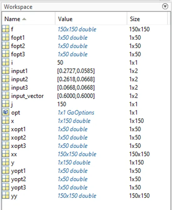
Results and Conclusion-
Following presented are the plotted curves and surfaces for studies 1, 2 and 3:
Figure (1):
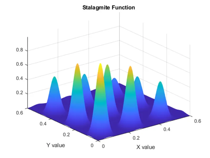
The following surface plot represents various local maxima for the following objective function for different values of ‘x’ and ‘y’.
Study 1: Unbounded random input sampling.
Figure (2):
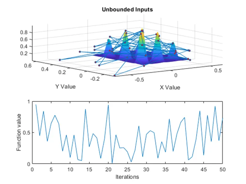
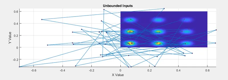
The plot shows various optimum solutions for the unbounded random input sampling for the values of ‘x’ and ‘y’. Since the input sample is random, negative values are also taken into consideration for input variables.
Study 2: Bounded input sampling.
Figure (3):
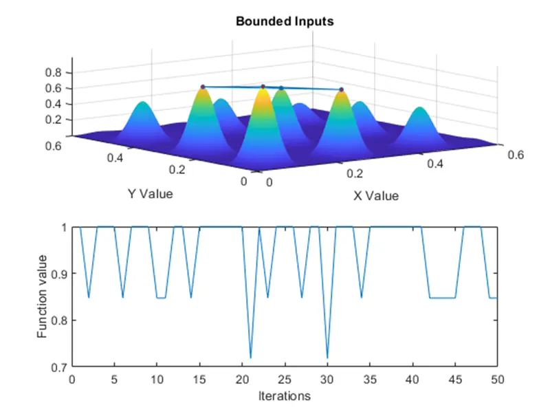
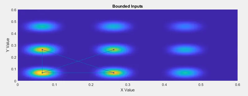
The plot shows the optimum solutions for various local maxima for respective ‘x’ and ‘y’ values. In order to restrict the sample size, the bounded method is used to limit the input variable’s range from 0 to 0.6.
Study 3: Bounded input sampling with additional optimization parameters.
Figure (4):
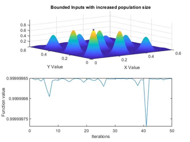
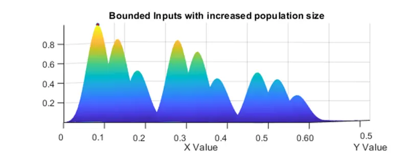
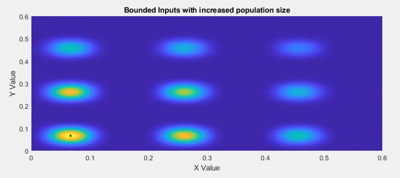
The following surface plots represent the objective function's global maxima and optimized solution. Since the program presented several local maxima, increasing the population and generation size also results in a higher probability of solution convergence towards global maxima.
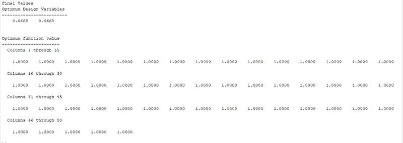
Therefore, the global maxima value for the following objective function is '1' and the optimum design variables values are x = 0.0668 and y = 0.0668.