Week 4.1 - Genetic Algorithm

OBJECTIVE :- To write a MATLAB code on Genetic Algorithm.

PROBLEM STATEMENT :-

Try to understand the concept of GA by reffering to various sources before you attend this challenge. Look out for information regarding stalagmite function and ways to optimize it.

• Write a code in MATLAB to optimize the stalagmite function and find the global maxima of the function
• Clearly explain the concept of GA in our own words and also explain the syntax for ga in MATLAB in our report.
• Make sure that our code gives the same output, even if it is made to run several times.
• Plot graphs for all 3 studies and for F maximum verses no. of iterations. Title and axes labels are a must, legend could be shown if necessary.

Content expected in the report-

1. Step wise explaination of your code
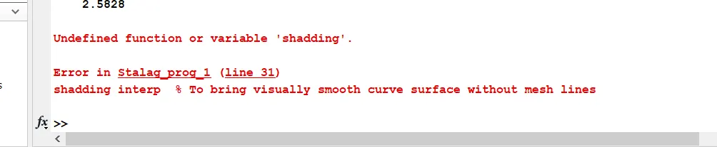
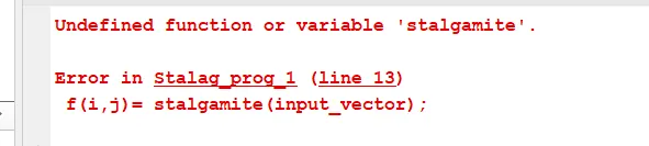
2. Mention the error while programming
3. steps taken to overcome those errors
4. Screenshot showing errors thrown in command window

THEORY & INTRODUCTIONS :-

The genetic algorithm is inspired by the process that drives biological evaluation. The process of evaluation starts with the selection of fittest individuals from a population. Then they produce offspring which inherrit the charecterastics of the parents and will be added to the next generation. If parents have better fitness, their offspring will be better than parents and have a better chance at surviving. This process keeps on iterating and at the end, a generation with the fittest individuals will be found. And this is the main working principle for the algorithm because at each step, the genetic algorithm selects randomly from the current populations tobe parents and uses them to produce the children forthe next geeratio.Over successive generations, the population evolves towards an optimal solution. The genetic algorithm can be applied to solve a variety of optimization problems that are not well suited for standard optiization algorith, including problems i which the objective function is discontinuous, nondifferentiable, stachastic or highly nonlinear.

The genetic algorithm uses three main types of rules at each step to create the next generation from the current population:

• Selection rules select the individuals, called parents that contribute to the populations at the next generation.
• Crossover rules combine two parents to form children for the next generations.
• Mutation rules apply random changes to individual parents to form children.

Algorithm Working Sequence :-

Algorithm then creates a sequence of new populations. At each step, the algorithm uses the individuals in the current generation to create the next population. To create the new population, it uses the fitness function which is the function you want to optimize.For standard optimization algorithms, this is known as the objective function.The toolbox software tries to find the minimum of the fitness function.

The algorithm performs the following steps-

• The algorithm begins by creating a random initialpopulations
• Then it scales the raw fitness scores to convert them into a more usable range of values. These scaled values are called expectation values.
• Then it selects members,called parents, based on their expectations.
• Along the individual that have high fitness value, some of the individuals i the current population that have lower fitness are chosen as elite. These elite individuals are passed to the next populations. Also it produces children by making random changes to a single parents-mutation-or by combining the vector entries of a pair of parents-crossover.
• It then replaces the current population with the children to form the next generation.
• Then it scores each member of the current population by computing it's fitness value. These values are called the raw fitness scores
• then the algorithm stops when one of the stopping criteria is met

fig. Mechanism for producing children

fig. Final answer developing with iterations.

Input Function :-

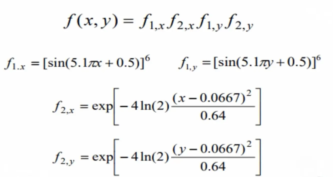
The above equations are used in the stalagmite function to plot the graph in the main functions-

function [f] = stalagmite(input_value)

f1x = (sin(5.1*pi*input_value(1) + 0.5)).^6;

f1y = (sin(5.1*pi*input_value(2) + 0.5)).^6;

f2x = exp(-4*log(2)*(((input_value(1) - 0.0667).^2)/(0.64)));

f2y = exp(-4*log(2)*(((input_value(2) - 0.0667).^2)/(0.64)));

f = -(f1x*f1y*f2x*f2y);

end

While using the function at the end as we are using the -ve sign so that the plot will be reversed as we have to find the maxima of the given function using ga.

Main Body :-

• Firstly creating the mesh from the two vectors which will be acting as a search space to find the maxima of the function.
• Creating the mesh of these two vectors using the 'mesh' command and defining the number of iterations as 'num_cases' to iterate the values of the optimum values of the function.
• Now calculating the values of fitness function at each point of the mesh grid formed.
• Now creating the values of fitness function at each point of the mesh grid formed.
• Now creating its surface through 'surfc' command which will also provide the contour of the generated surfaces.
• While using surfcapplying the -ve sign to the function will generate the surface upside down which will be quite good to get the maxima of the function, as it will provide positive value for the maxima using the -ve sign.

STEP BY STEP CODING PROCEDURE :-

1. First, Linspace command is used to define x & y with 150 elements between zero and 0.6 including the bounds.
2. Then num_cases is set which will be used as counter for iteration to 50
3. then a 2D grid is made using meshgrid command is created from x & y input tobe output to xx & yy
4. then for loop is used to solve the genetic algorithm for every element in the 2D mesh grid
5. the length of rows & column (which have equal length) are used as counters
6. then the input vector is declared as ga requires input vector which is each value in the mesh grid
7. then output of stalagmite function is stored in matrix
8. then tic command is used to start a timer
9. then for loop bounded by the number of iterations is formed
10. then ga code is entered for unbounded statistical study which have the following format :

[inputs, fopt] = ga(fun, nvars)

inputs represent the values of parameters x & y for which the function has the least value (fopt)

fun - the function tobe optimized, in this case stalagmite

nvars - the number of design variables, in this case only x & y are the variables tobe plotted

11. Then smallest (minimum) value of the function for each iteration is output & its x & y coordinates which are stored in seperate variables

12. then 'toc' command is used to stop the timer and the output is stored in study_time1

13. then figure1 is plotted by the following steps-

14. First subplot command is used to partition the plot window in order to draw more than one plot in the same window, two rows and one column are specified and then the position of each plot is selected

15. then hold on command is used to prevent plot for being removed

16. the surfc command is used to plot contour with xx & yy value from the mesh grid as input and negative optimum value is used because we need to maximize the function

17. then x,y,& z axis are labelled

18. then shading interp is used to smoothen the function plot and to remove the grid lines

19. then plot 3 command is used to plot a point in 3D, here it will plot- fopt because we need the maximum value of the function not the minimum

20. then the graph title is selected

21. then fopt value of the function is plotted on the second plot in the second row

22. then its x & y axis are labelled.

23. then the same study is made but this time it is bounded (has lower & upper limit) which requires the same commands and step excepts the ga command which have the following format :

[input, fopt] = ga(fun, nvars, A, b, Aeq, beq, lb, ub)

Inputs, fopt, fun & nvars are the same as study-1

A - Linear inequality constraints : real matrix, if there are none, then []

b - Linear inequality constraints : real vector, if there are none, then []

Aeq - Linear equality constraints - :- real matrix, if there are none, then []

beq - Linear equality constraints - real vector, if there are none, then []

lb - lower bounds, specified as a real vector or array

ub - upper bounds, specified as a real vector or array

24. the range of the genetic algorithm is bounded by introducing values for lower and upper bounds and hence the values of global maxima and the values of x & y will be within the defined search space in inputs

25. then increasing population size study was done which is the same as before but it had different ga code of :

[inputs, fopt] = ga(fun, nvars, A, b, Aeq, beq, lb, ub, nonlcon, IntCon, options)

inputs, fopt, fun and nvars, A, b, Aeq, beq, lb, ub are the same as study-1 and study -2 respectivelly

nonlcon - nonlinear constraints, specified as a function handle or function name. If there are none then []

IntCon - Integer variables, specified as a vector of positive integers, if there are none, then []

Options - Optimization options, specified as the output of optimoptions or a structure.

26. the range of the genetic algorithm is bounded as in study-2 but to improove the accuracy, the commands optimoptions is introduced to increase the Population Size

27. then total time is computed

28. then using fprintf command the results are printed in the command windows

29. then the study time is printed

30. then x, y coordinate of the maximum optimum values are printed

31. then the optimum values of the function (maximum value) is printed which is calculated from the (negative mean) of the all iterations of the output value and the negative sign is used to get the maximum value

32. then the study time of the whole 3 studies combined is printed.

MATLAB CODE :-

clear all 
close all
clc

x = linspace(0,0.6,150);
y = linspace(0,0.6,150);
num_cases = 50;

% creating a 2D mesh
[xx,yy] = meshgrid(x,y);

%Evaluating Stalagmite function
for i = 1:length(xx)
    for j = 1:length(yy)
        input_value(1)=xx(i,j);
        input_value(2)=yy(i,j);
        f(i,j) = stalagmite(input_value);
    end
end

% Study1- Unbounded statistical behaviour
tic
for i = 1:num_cases
    [inputs1, fopt1(i)] = ga(@stalagmite, 2);
    xopt(i) = inputs1(1);
    yopt(i) = inputs1(2);
end
study1_time = toc;

figure(1)
subplot(2,1,1)
hold on
surfc(xx,yy,-f)
xlabel('X-Values')
ylabel('Y-Values')
zlabel('Function Values')
shading interp
plot3(xopt,yopt,-fopt1,'marker','o','markersize',5,'markerfacecolor','r')
title('Unbounded Statistical Behaviour')
subplot(2,1,2)
plot(-fopt1)
xlabel('Iterations')
ylabel('Function maximum')

% Study2 - Statistical behaviour with upper aned lower bound
tic
for i = 1:num_cases
    [inputs2,fopt2(i)] = ga(@stalagmite,2,[],[],[],[],[0;0],[1;1]);
    xopt(i) = inputs2(1);
    yopt(i) = inputs2(2);
end
study2_time = toc

figure(2)
subplot(2,1,1)
hold on
surfc(xx,yy,-f)
xlabel('X-Values')
ylabel('Y-Values')
zlabel('Function Values')
shading interp
plot3(xopt,yopt,-fopt2,'marker','o','markersize',5,'markerfacecolor','r')
title('Bounded Statistical Behaviour')
subplot(2,1,2)
plot(-fopt2)
xlabel('Iterations')
ylabel('Function Maximum')

%Study3- increasing GA iterations (Population size)
options = optimoptions('ga');
options = optimoptions(options,'PopulationSize',170);

tic
for i = 1:num_cases
    [inputs3, fopt3(i)] = ga(@stalagmite,2,[],[],[],[],[0;0],[1;1],[],[],options);
    xopt(i) = inputs3(1);
    yopt(i) = inputs3(2);
end
study3_time = toc

figure(3)
subplot(2,1,1)
hold on
surfc(xx,yy,-f)
xlabel('X-Values')
ylabel('Y-Values')
zlabel('Function Values')
shading interp
plot3(xopt,yopt,-fopt3,'marker','o','markersize',5,'markerfacecolor','r')
title('Bounded Statistical behaviour with modified population size')
subplot(2,1,2)
plot(-fopt3)
xlabel('Iterations')
ylabel('Function maximum')

Total_time = study1_time + study2_time + study3_time
fprintf('n The results are below : ')

fprintf('nn study 1 : Unbounded statistical Bahaviour')
fprintf('nn The time taken for the study-1 is : %f',study1_time)
fprintf('n The co-ordinates of x & y for the global Maxima of the function are : %f,%f',inputs1(1),inputs1(2))
fprintf('nn the global maxima of the  function is : %f',-(mean(fopt1)))

fprintf('nn study 2 : Unbounded statistical Bahaviour')
fprintf('nn The time taken for the study-2 is : %f',study2_time)
fprintf('n The co-ordinates of x & y for the global Maxima of the function are : %f,%f',inputs2(1),inputs2(2))
fprintf('nn the global maxima of the  function is : %f',-(mean(fopt2)))

fprintf('nn study 3 : Unbounded statistical Bahaviour')
fprintf('nn The time taken for the study-3 is : %f',study3_time)
fprintf('n The co-ordinates of x & y for the global Maxima of the function are : %f,%f',inputs3(1),inputs3(2))
fprintf('nn the global maxima of the  function is : %f',-(mean(fopt3)))

OUTPUT :-

Unbounded Statistical Behaviour Plot :- (Iterations = 50)

In this above image it can be seen that since the inputs are boundless GA algorithm has mapped local maxima points outside our stalagmite function. Also we can not infer a particular value of global maxima from the above graph, and it is hence pointless.

The study time is very less as the 'ga' algorithm is made only to run for 50 iterations.

Bounded Statistical Behaviour Plot :- (Iterations = 100)

The above graph is more clear and optimized compare to the first iterations since here the bounds were defined and we could get only the values within our range. We are now more clear on the range within which our maxima lies.

Modified Population Size Plot :- (Iterations = 170)

In this case we are getting the optimized value of global maxima with accurate range, since we increased the number of iterations and population size.

Since the number of iterations and population size is increased the study time is so high compared to the previous two iterations.

Thus it can be concluded that GA gives more accurate results in case of bounded inputs and by increasing the number of iteration and population size.

It can also be infered that even if we define a particular search space for GA, the GA doesn't run inside the search space. Only in casses of bounded inputs we can get interfearable results.

Stalagmite Function Output print in Command Window :-

Errors While Programming :-

1.

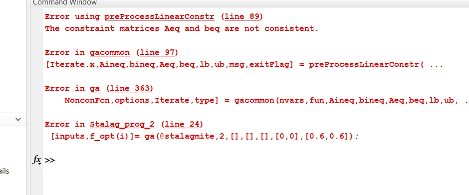
The error was in the GA algorithm syntax, wherein I did not type a '[]'.

2

.

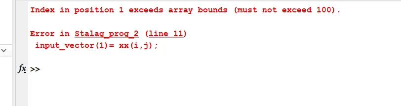
While defining the inputs mention different sizes of input vectors x & y. The error is basically due to the mesh grid command where in the two vectors cannot be combined due to their varying sizes.

3.

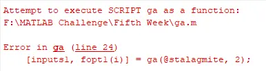
this error occurs because of my file name same as that of inbuilt function in MATLAB.

Apart from these some types of error are-

CONCLUIONS :-

1. Unbounded statistical Behaviour-

The time taken for the study-1 = 5.912489 sec

The global maxima of the function = 0.512086

2. Bounded statistical behaviour-

Time taken for the study-2 = 7. 937613 sec

The global maxima of the function = 0.905461

3. Bounded statistical behaviour with increase population size -

Time taken for the study-3 = 19.544688 sec

The global maxima of the function = 0.993887

The total time taken to complete the total study = 33.305790

Refferences :-

1. https://en.wikipedia.org/wiki/Genetic_algorithm
2. https://towardsdatascience.com/introduction-to-genetic-algorithms-including-example-code-e396e98d8bf3
3. https://www.geeksforgeeks.org/genetic-algorithms/