Week 4.1 - Genetic Algorithm

introduction :

Genetic algorithm is derived from charles darwins theory of evolution which states that it is not the strongest of the species that survies nor the most intelligent but the one most responsive to change the entire concept of genetic algorithm is based on the above famous statement.

Genetic Algorithm is only used to generate minimum solution so the value of stalagmite function is taken negative to maximise the function.

syntax for ga:

x = ga(fun,nvarsA,b,Aeq,beq,ib,ub)

where,

1)x= optimum solution/variables.

2)no_of_variables = nyumber of variables,specified as a positive integer.

3)A,b linear inequality constraints.

4)Aeq,beq = linear bounds,ub=upper bounds

6)nonlcon:use for nonliner constration.

7)intcon:to get solution in integer.

8)options:minimize with non default options.

Matlab Code:

Stalagmite Function Code

function [f] = stalagmite(input_vector)

x=input_vector(1) ;
y=input_vector(2) ;

f1=(sin(5.1*pi.*x+0.5)).^6;
f2=(sin(5.1*pi.*y+0.5)).^6;
f3=exp(-4*log(2).*(((x-0.0667).^2)/0.64));
f4=exp(-4*log(2).*(((y-0.0667).^2)/0.64));

f=-(f1.*f2.*f3.*f4);

end

program

clear all
close all
clc

% Defining our search space
x = linspace(0,0.6,150);
y = linspace(0,0.6,150);

% Creating a 2Dimensional mesh
[xx yy] = meshgrid(x, y);

% Evaluating the stalagmite function
for i = 1:length(xx)
    for j = 1:length(yy)
        inputs_vector(1)=xx(i,j);
        input_vector(2)=yy(i,j);
        f(i,j) = stalagmite(input_vector);
    end
end



surface(xx,yy,f)

%shading interp


[x, fval] = ga(@stalagmite, 2)

% Defining our search space
x = linspace(0,0.6,150);
y = linspace(0,0.6,150);

% Creating a 2Dimensional mesh
[xx yy] = meshgrid(x, y);

% Evaluating the stalagmite function
for i = 1:length(xx)
    for j = 1:length(yy)
        inputs_vector(1)=xx(i,j);
        input_vector(2)=yy(i,j);
        f(i,j) = stalagmite(input_vector);
    end
end



surface(xx,yy,f)

shading interp


[x, fval] = ga(@stalagmite, 2)

% Defining our search space
x = linspace(0,0.6,150);
y = linspace(0,0.6,150);

% Creating a 2Dimensional mesh
[xx yy] = meshgrid(x, y);

% Evaluating the stalagmite function
for i = 1:length(xx)
    for j = 1:length(yy)
        input_vector(1)=xx(i,j);
        input_vector(2)=yy(i,j);
       f(i,j) = stalagmite(input_vector);
    end
end



surfc(xx,yy,f)
xlabel('x value')
ylabel('y value')

shading interp


[inputs, fval] = ga(@stalagmite, 2)

function [f] = stalagmite(a)

x = a(1);
y = a(2);

f1=(sin((5.1*pi*x)+ 0.5)).^6;
f2=(sin((5.1*pi*y)+ 0.5)).^6;
f3=exp((-4*log(2)*((x-0.0667).^2))/(0.64));
f4=exp((-4*log(2)*((y-0.0667).^2))/(0.64));

f=-(f1.*f2.*f3.*f4);

end

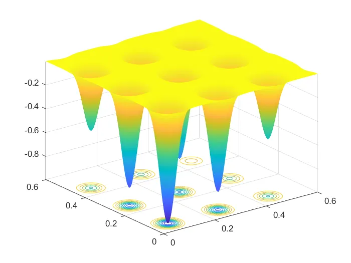
study 1 plot:

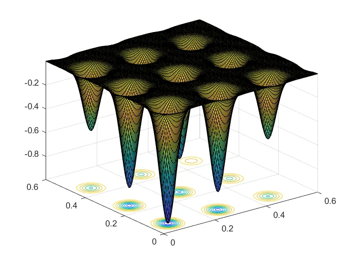
study 2 plot

study 3 plot

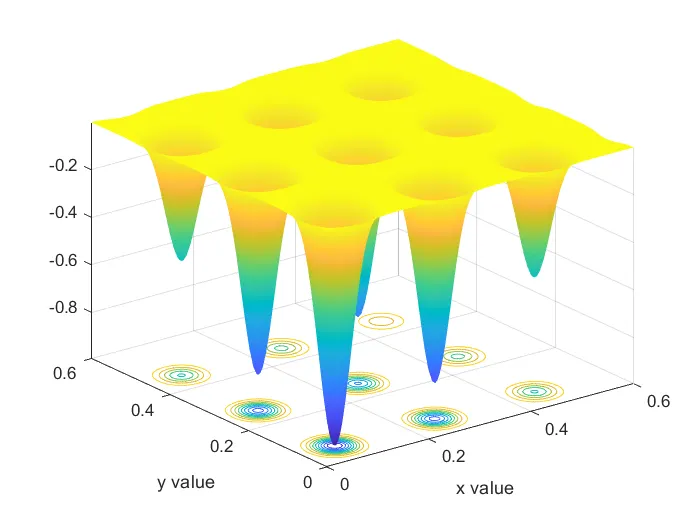
this point on the peak is called the global maxima

Results and conclusions:

hence by using generic algorithm we were able to find the global maxima point of the stalagmite function

by default in matlab ga calculation the global minima in order to make it show the global maxima we add a ve sign to f and fopt everyehere

initially the time required to run the program is long we can reduce this time by reducing the limits decreasing the population size will get more accurate results

report

1 intially creat x and y array and number of iterations you want

2 study -1 it calulate the global maxima by taking random samples from the function calculating the time taken for study 1

3 syntax for ga in study-1 is

[inputs,fopt(i)]=ga(@stalagmite,2);

4 study 2 it calculate the global maxima by giving boundary limits for the inputs

5 syntax for ga in study-2

[inputs,fopt(i)]=ga(@stalagmite,2,[],[],[],[0;0],[1;1];,in that you see the boundary limits 0 to 1.

6 study 3 it calculate the global maxima by giving population size by which we can find the specific optimum point

7 syntax for ga in study -3

[input,fopt(i)]=ga(@stalagmite,2,[],[],[],[0;0],[0.6;0.6]options);